Deep Feature Matching

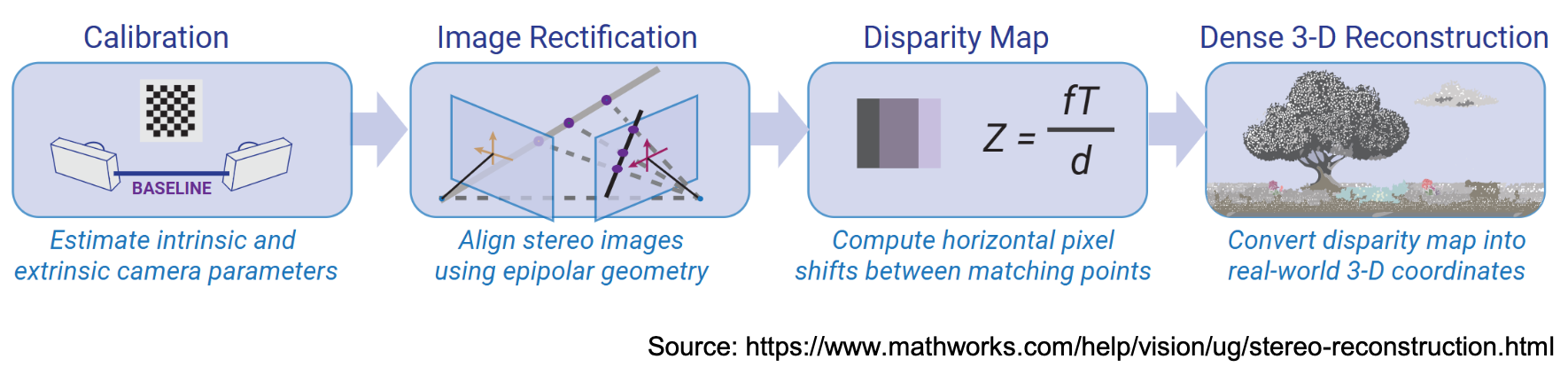
Stereo I haven’t done so far. However, 3D Indoor Reconstruction, camera calibration and 3d recontruction, Bundle Adjustment are all topics that have a somewhat connection to it. Stereo is basically seeing a 3D point from two different POVs (rays), which enables us to use triangulation in order to get the disparity map ⇒ depth (since it’s the inverse).

Stereo cameras deliver scaled scenes ⇒ metric depth is recoverable. Monocular cameras cannot do this without additional assumptions. Typical robot applications: collision avoidance, 3D environment mapping, semantic scene understanding.

Ok but what does "scaled scene" mean?

When you have a stereo camera, you know the physical baseline — the real-world distance between the two lenses (say, 10 cm). So when you compute disparity and apply

$$Z=\frac{B\cdot f}{disparity}$$

the B in that formula is an actual metric value in meters. The depth Z you get out is therefore also in real meters.

• With a mono camera, you have no baseline. If you move the camera and try to reconstruct depth from two frames, you can compute the relative motion and relative depth — but you cannot recover the absolute scale.
• This is why in self-supervised monocular depth (SIDE), the PoseNet co-estimates camera motion but the depths must be normalized — you only recover depth up to an unknown scale factor. You know object A is twice as far as object B, but not whether A is 2m or 20m away.

The mathematics can be found in Depth Accuracy For Stereo Cameras. I should also look again over these notes on SfM vs Dense Matching.

Challenges include reflective or transparent surfaces (no stable texture to match), half-occlusions (regions visible in one camera and hidden in the other), shadows.

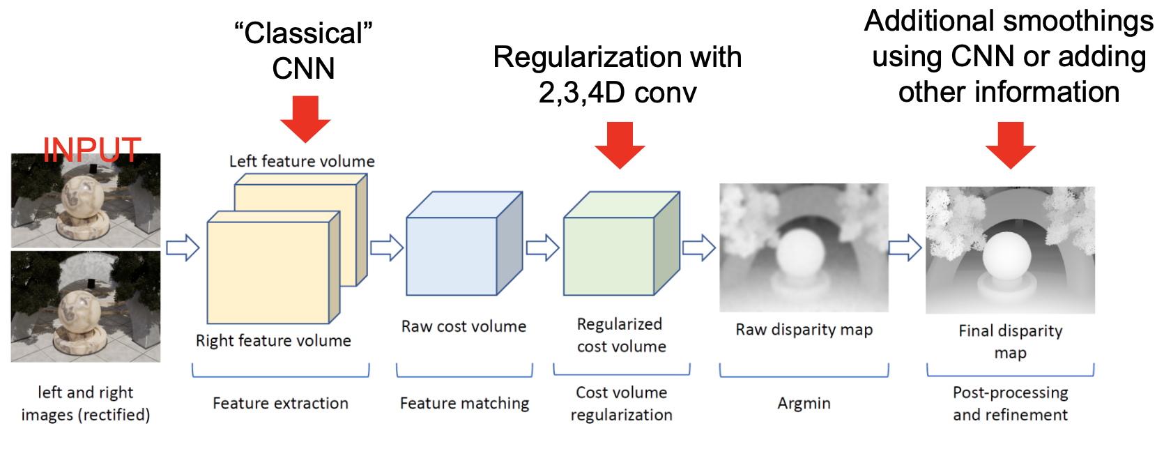
Deep Feature Matching for 3D Stereo Reconstruction

Classical stereo used handcrafted descriptors (SIFT, ORB — see Deep Learning SfM, SLAM, and VO). The DL approach learns to match directly from data, replacing one or more stages of the classical pipeline.

Challenges remain the same.

The pipeline remains

$$\text{feature extraction}\to \text{feature matching}\to disparity\to \text{post-processing}$$

• DL replaces the first two steps with a CNN, adds 2D/3D/4D convolutional regularisation on the cost volume, and optionally adds a final CNN-based refinement.

Siamese Networks are the fundamental architecture for learned stereo matching: two branches with shared weights, one for each image patch.

Siamese Network Architecture

1. Two image patches are fed into parallel convolutional towers.
2. Each tower produces a feature vector (Conv $\to$ ReLU $\to$ MaxPool $\to$ $\dots$)
3. Similarity is scored either by a decision network (MLP on concatenated features, more accurate, slower) or by a dot product after normalisation (faster, requires lifting features to the same space).

Fusion between the two branches can happen at different points: early fusion (concatenate raw inputs), middle fusion (concatenate mid-level features), or late fusion (merge final descriptors). Each trades off accuracy against speed.

Importantly, the Siamese approach produces a sparse reconstruction — one correctly matched patch gives one 3D point. For dense depth maps, the process must iterate over all pixels or be replaced by a global approach (use of attention layers to have more context, or multi-scale approach).

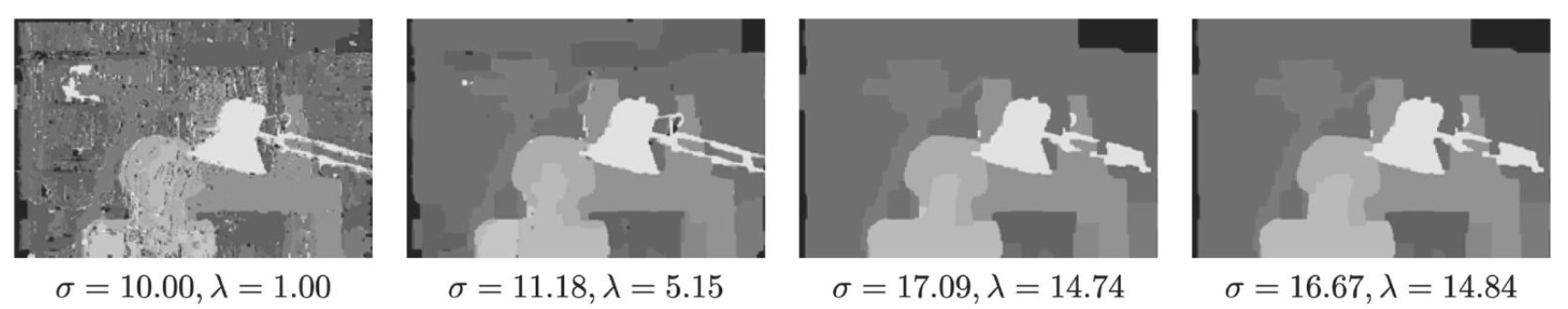
Spatial Regularization — MRF

MRF regularization improves disparity map by spatially smoothing while preserving important discontinuities.

MRF cost

The idea remains as in SIDE — neighboring pixels should usually have similar depth, unless there is evidence of an edge or object boundary

The energy to minimize is:

$$E(d)=\sum _i{D}_i(d_i)+\lambda \sum _{i,j}V(d_i,d_j)$$

The data term $D_i$ measures how well disparity $d_i$ explains the observed stereo match; the pairwise term $V$ penalises large disparity differences between neighbouring pixels. The four depth maps in the slide show the effect of increasing $\lambda$ — smoother at higher $\lambda$ but at risk of over-smoothing edges.

Training Strategies

Again 3 options.

• Supervised: Minimise discrepancy between predicted and ground-truth matching scores/disparities for each sample. Training with patch triplets: one reference patch, one positive match (correct disparity), one negative match (wrong disparity). The loss enforces $sim(f_L,f_{+})>sim(f_L,f_{-})$. In general, the loss functions have these elements:
  • a confidence term $C(x)$
  • a Heaviside function — only include this pixel in the loss if its confidence $C(x)$ exceeds threshold $ϵ$
  • a log-space distance measure (helps manage short and long distances jointly)
  • the estimated vs ground-truth depth difference

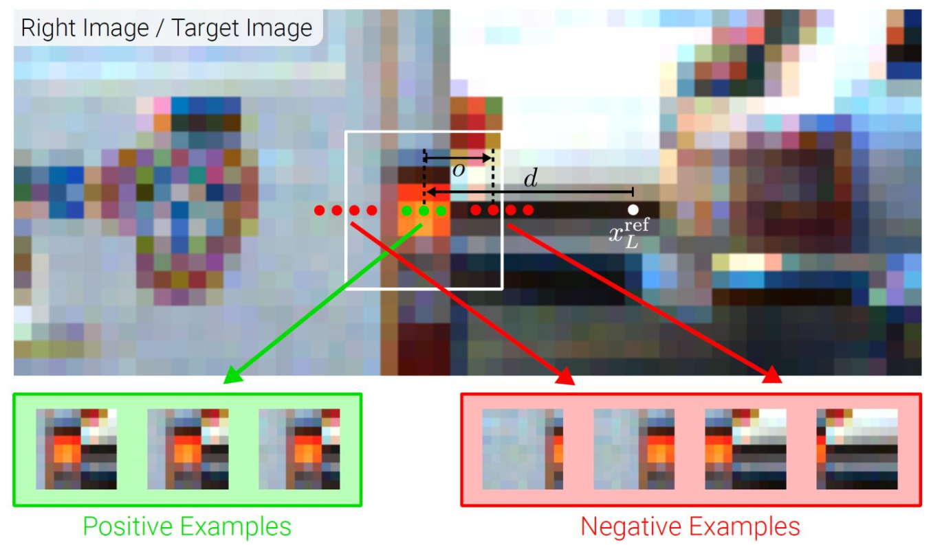
• Weakly supervised: Instead of one labelled positive patch, the model is given the full set of candidate patches along the epipolar line. These methods are motivated by the reduced amount of real ground-truths. The constraints that replace explicit labels:

1. Epipolar constraint — the correct match lies on the same scanline after rectification.
2. Disparity range — match must be within a valid interval.
3. Uniqueness — one pixel matches at most one pixel.
4. Continuity / smoothness — neighbouring pixels have similar disparity.
5. Ordering — matches preserve left-to-right order (except near occlusions).

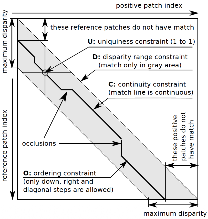
Loss combinations used: Multi-Instance Learning (MIL) — best positive must score higher than best negative; contractive loss — adds uniqueness; contractive-DP — uses all constraints and finds the best match via dynamic programming.

An important quality signal: left-right consistency check -- reconstruct the scene swapping the order of left and right images and compare. Inconsistencies expose unreliable matches. This consistency can also be embedded in a recurrent model where two depth maps cross-check each other iteratively.

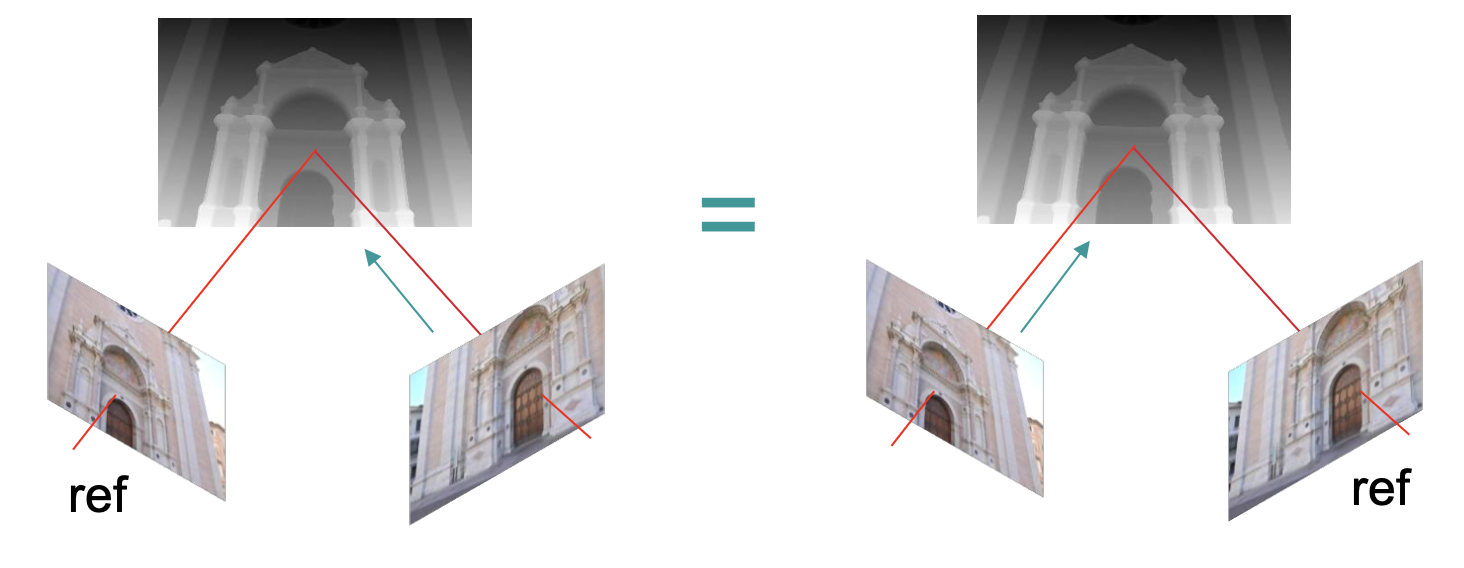
• Self-supervised: If the 3D reconstruction is correct, un-warping the right image into the left viewpoint using the estimated depth should reproduce the original left image. The loss is:

$$Loss=\frac{1}{N}\sum D(\varphi (I_{ref})(x)-\varphi ({\hat{I}}_{ref})(x))$$

Distance measure D can be photometric error, a learned feature map distance, or an image-gradient loss.

As mentioned in SIDE, all three training paradigms can be enriched with:

• Smoothness — penalize large disparity variation in homogeneous regions.
• Consistency — the left-right reconstruction symmetry.
• Scale-invariant gradient losses — smoothness of gradients in the neighbourhood.
• Incorporating semantic cues — use normal, segmentation, and edge maps to guide disparity estimation. Growing in popularity with 3D semantic mapping.

Domain Adaptions

Training data strongly determines performance. Ground truth is expensive — usually from structured light, LiDAR, or manual annotation. Strategies to bridge the gap:

• Sparse + reliable point clouds — even a few thousand LiDAR points can anchor the scale (so ground truth data).
• Synthetic datasets — are also emerging and promise to replace the need for real datasets in many applications. Increasingly replaced by generative AI rendering. Saw them in one NVIDIA post. Also a topic at TNO I talked in one interview.
• Foundation model pre-training — DINOv2 can also help to pre-train parts of the model.