Deep Learning SfM, SLAM, and VO

Feature matching — blobs

Blobs are regions with positive or negative brightness or colour value compared to their neighbourhood

1. First, images are filtered to simulate different scales (e.g. Gaussian Blurring) ⇒ scale-space representation
2. Filtered image at one scale is subtracted from filtered image at previous scale
3. Check for local extrema across scales

Feature matching — descriptors and similarity measures

SIFT

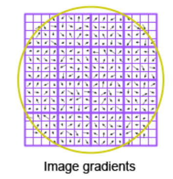
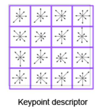
1. A $16\times 16$ pixel neighbourhood around an identified feature point (also keypoint) is selected
2. The orientations (simplified to 8 possible directions) of the gradients are computed for a $4\times 4$ array in a $16\times 16$ image region
3. Then, they are stored in a $4\times 4$ keypoint descriptor with 8 possible orientations which are weighted ⇒ 128 byte descriptor vector
4. Similarity is assessed considering the Euclidean distance

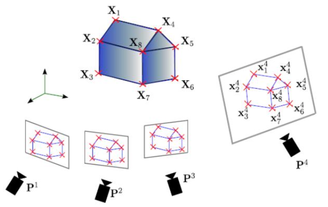
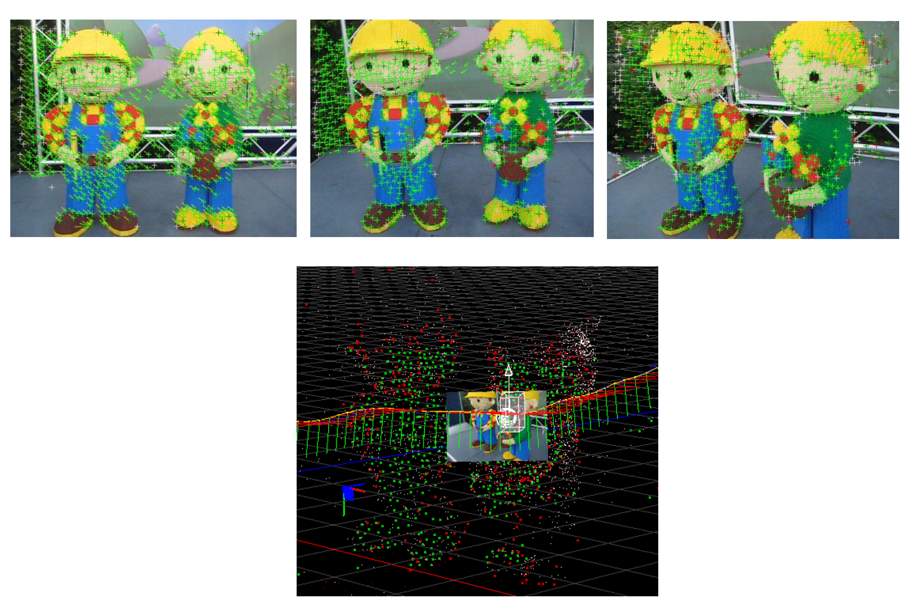
Triangulation is basically determining a 3D point in space given its projection onto two or more images. So these points are usually called tie-points. However, one question was asked during the lecture: how do we remove the wrong matches?

• RANSAC — the idea that you only select points within a small distance to a line you’re trying to fit (i.e. inliers). The concept is very similar to the Hough transform from Point Cloud Segmentation.
  • For all possible lines, select the one with the largest number of inliers.
• They suggest computing the fundamental matrix F based on the detected inliers.

Structure from Motion(SfM): SfM aims to reconstruct the 3D structure of a scene and the camera’s motion from a sequence of images. This is how they do the motion prediction in NeRF. In Gaussian Splatting, SfM is used to produce a sparse point cloud since it gives the corresponding camera poses.

• you need at least one camera and a set of overlapped images.
• you assume the scene is rigid.

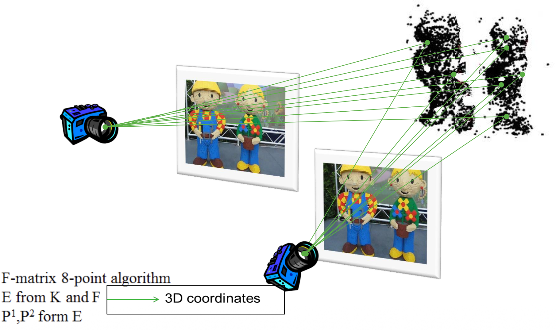
SfM - Practical Implementation

1. Match or track points over the whole image sequence.

2. Initialize the structure and motion recovery

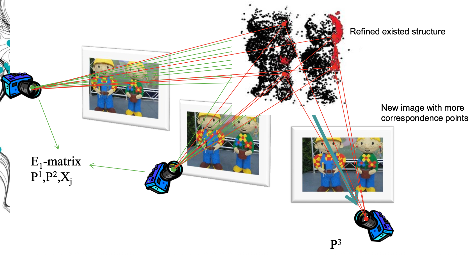
3. For every additional view infer matches to the structure and compute the camera pose and refine the existing structure.

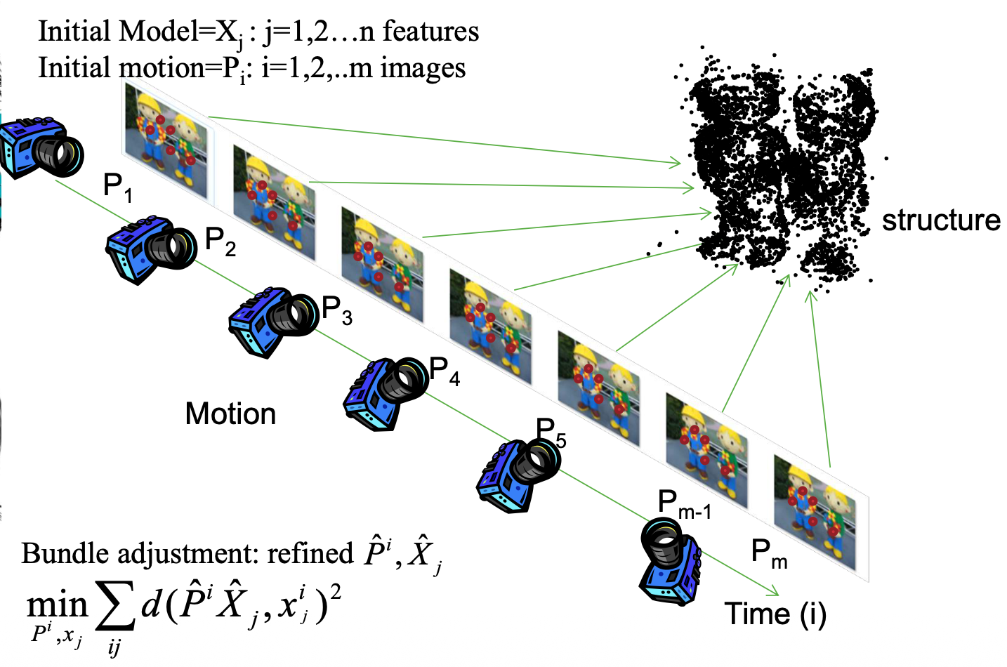
4. Refine the SfM through bundle adjustment

Visual Odometry is a particular case of SfM.

• it focuses on estimating the 3D motion of the camera sequentially (as a new frame arrives) and in real-time.
• several prerequisites are necessary like sufficient illumination and sufficient overlap between consecutive frames.
• BA can be used (but it’s optional) to refine the local estimate of the trajectory.

Sometimes, SfM is erroneously used as a synonym of VO

SfM is more general than Visual Odometry and tackles the problem of 3D reconstruction of both the structure and camera poses from unordered image sets.

The final structure and camera poses are typically refined with an offline optimization (i.e. bundle adjustment), whose computation time grows with the number of images!

Motion estimation — key frame selection: Several hundreds of frames can be acquired in few seconds of video. Most of the frames give similar information and they are maybe not useful for VO purposes.

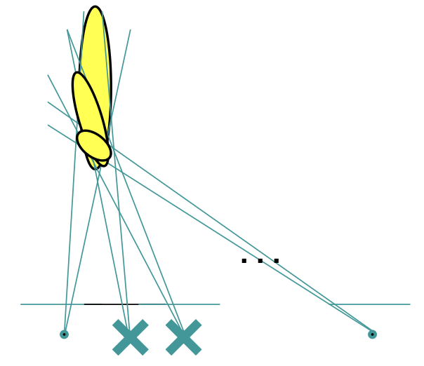
• When frames are taken at nearby positions compared to the scene distance, 3D points will exhibit large uncertainty.
  • As a consequence, 3D-3D motion estimation methods will drift much more quickly than 3D-2D and 2D-2D methods

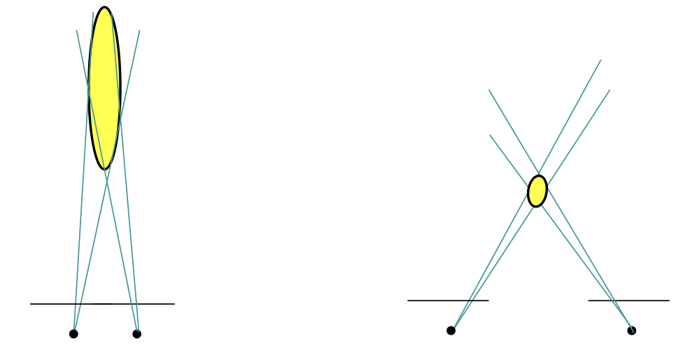
• One way to avoid this problem consists of skipping frames until the average uncertainty of the 3D points decreases below a certain threshold. The selected frames are called key-frames.

Stereo vision has the advantage over monocular vision that both motion and structure are computed in the absolute scale. It also exhibits less drift (at least in indoor environments). When the distance to the scene is much larger than the stereo baseline, stereo VO degenerates into monocular VO — idea also mentioned in PPROS and CONS of Sensor Configurations (the one with the poor ray intersection in a corridor).

We also talked of Loop Closure. The highlight was how to detect them. They introduced the Bag-of-words method which “summarizes” the information stored by all the descriptors in an image into a database that allows to quickly compare keyframes and detect similarities

Regarding SLAM, ORB-SLAM3 is apparently a widely used solution. Nice video on it.

• Tracks FAST features + ORB descriptors
• Can be visual or visual-inertial ⇒ combination to bridge gaps
• Place recognition, map merging and loop closure using bag of words

Direct methods do not extract features, but use directly the pixel intensities in the images, and estimate motion and structure by minimizing a photometric error.

• The depth map are not created for all the pixels, but only for those in the neighborhood of large image intensity gradients, making them semi-dense. LSD SLAM
• Three main steps:
  • Tracking
  • Depth map estimation
  • Map optimization

Deep Learning approaches for SLAM

Three different typologies of SLAM using DL can be catalogued (Monocular SLAM case):

• Supervised: ground truth is used to train the network. The CNN regress the camera pose and the depth.
• Self-supervised: the photometric loss is used to train without the need for ground truth. Image warping from one frame to another frame is used to determine the pose and minimize the loss by back-propagation
  • we can define the photometric loss as the difference between the warped image and the target image
• Hybrid supervision: many supervision labels such as the real pose, depth map that are used during the training to support the process.

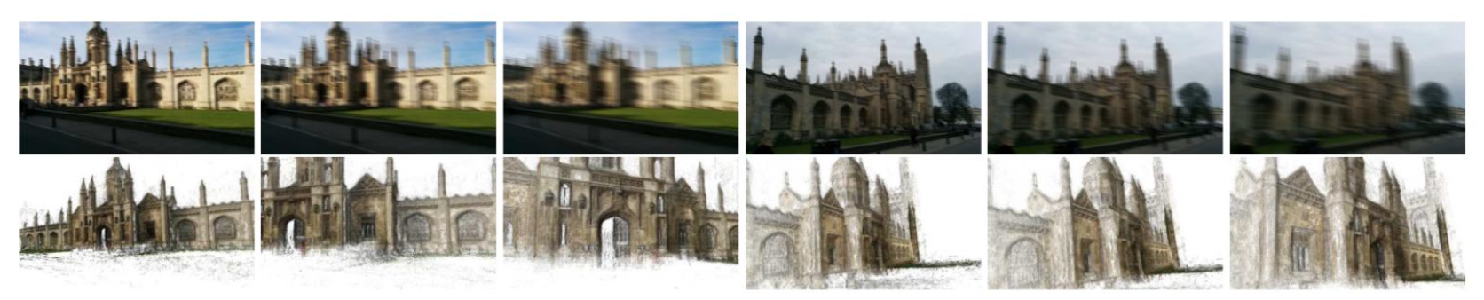
Stereo-pair pose estimation with DL: PoseNet — Compared to previous methods it simultaneously learns position and rotation. Camera pose is given by translations ($x$) and rotations ($q$, in quaternion form)

• Higher performances in challenging situations: blurred images, hard weather conditions $\to$ able to see contours and homogenous areas
• Still relatively low accuracies. On GPU, faster than traditional algorithms
• The system is robust to wider baselines between images

Conventional methods vs DL ones

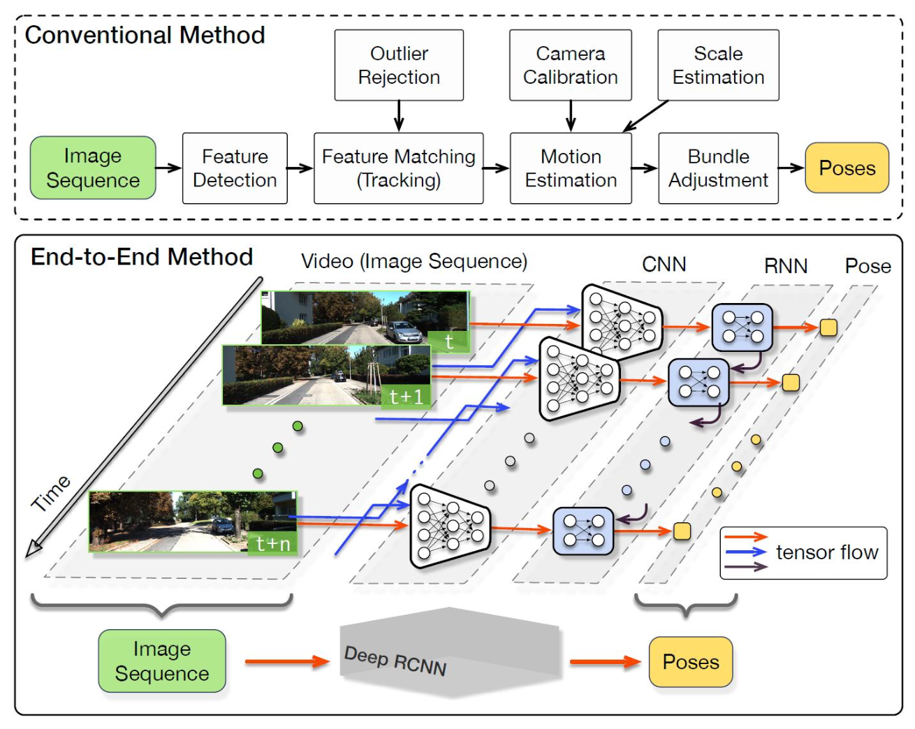
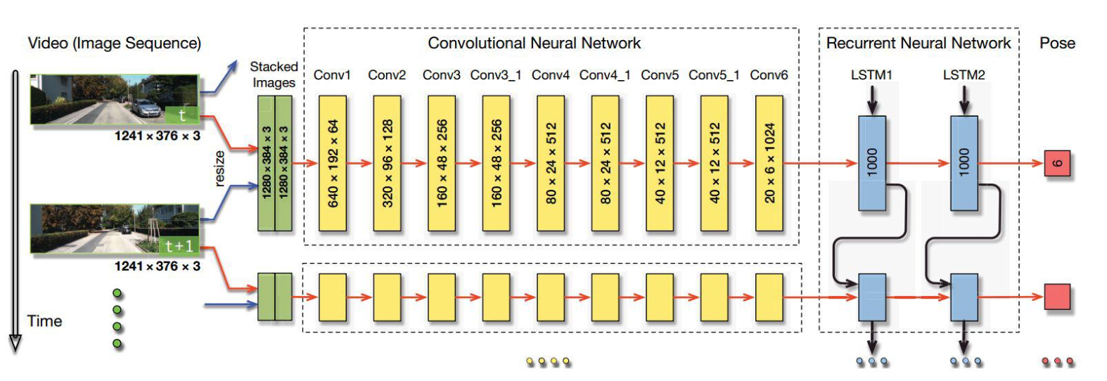
DeepVO is a supervised method.

• Initial convolutions on two stacked images to derive features
• Use of RNNs (LSTM) to keep the connection among consecutive images
• often has overfitting problems
• Results are strongly influenced by the length of the training sequence
• Scale can be learnt during the end-to-end training

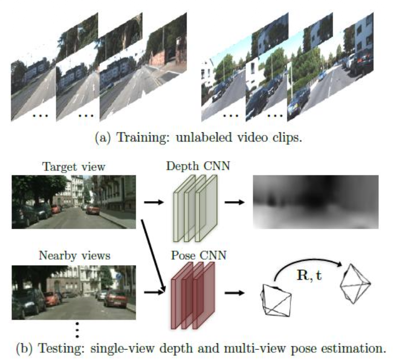
SfMLearner is a self-supervised method which combines a depth model and a pose estimation model and embeds projective geometry in the learning process.

DVSO is a hybrid method combining deep learning depth prediction and traditional direct sparse odometry (DSO) results. The training combines depth predictions given by traditional (i.e. DSO) and DL methods.

Three elements:

1. self-supervised learning from photo consistency
2. supervised learning based on traditional direct methods
3. Stacknet for monocular depth estimation

A growing trend in the use of DL to estimate depths is:

• ORB SLAM + Single image depth estimation to densify the 3D reconstruction i.e. densification.

Loop closures with DL:

• Researchers have proposed to use the ConvNet features, that are from pre-trained neural models on large-scale generic image processing dataset. Image similarity is calculated with the norm of the feature vector to determine whether a loop exists.
• Another approach is to use deep auto-encoder structure to extract a compact representation, that compresses the scene in an unsupervised manner.
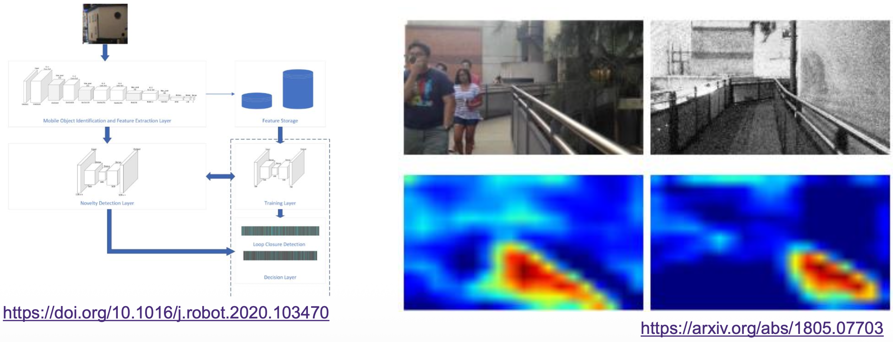
• Other specific networks have been designed to quickly detect if that region has been visited or not (novelty networks) combining it with “dictionary” that stores the information of previous frames.

Windowed Bundle Adjustment with DL

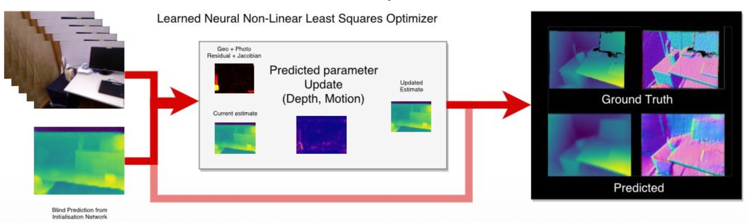
• LS-Net tackles this problem via a learning-based optimizer by integrating analytical solvers into its learning process.
  • It learns a data-driven prior that is then improved by refining neural network predictions with an analytical optimizer to ensure photometric consistency.
  • It can optimize sum of squares objective functions in SLAM algorithms, which are often difficult to optimize due to violated assumptions and ill-posed problems.

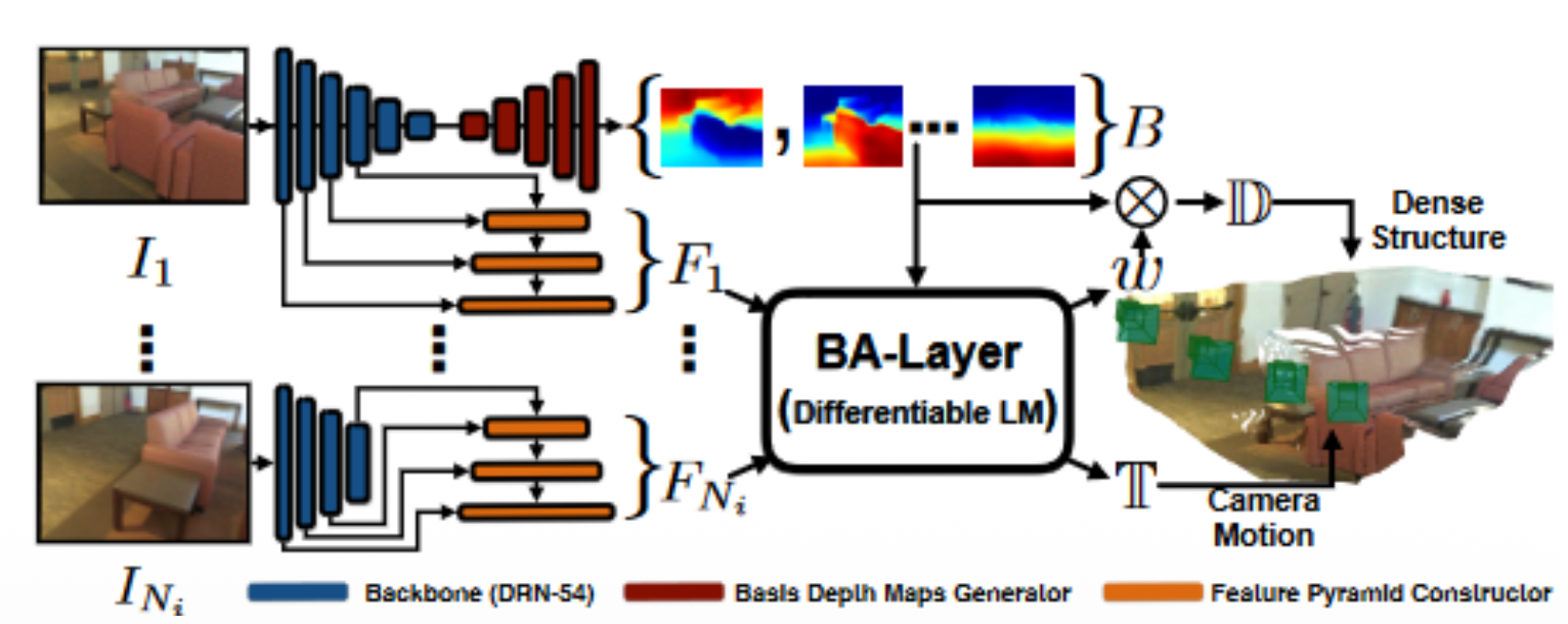
• BA-Net integrates Levemberd Marquardt into a deep neural network for an end-to-end learning.
  • Instead of minimizing geometric or photometric error, BA-Net is performed on feature space to optimize the consistency loss of features from multi view images extracted by ConvNets.
  • The feature-level optimizer can mitigate problems of geometric or photometric solution (e.g. some information lost in the geometric optimization, while environmental dynamics and lighting changes may impact the photometric optimization).

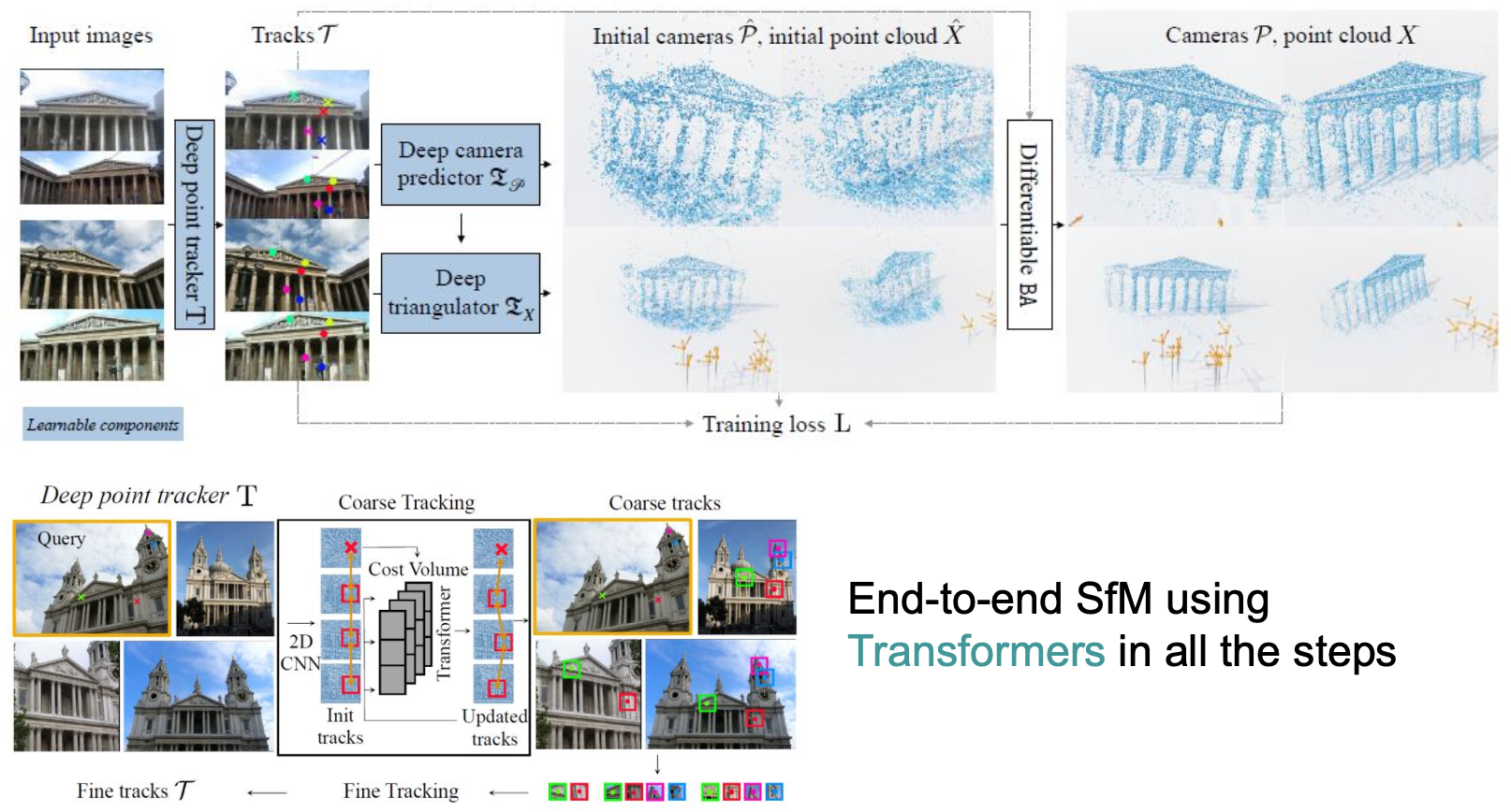
VGGSfM — Visual Geometry Grounded SfM

• Coarse-to-fine feature tracking: coarse estimate and confidence prediction is used to guide fine tracking on smaller regions
• The initial positions of cameras and 3D points are then refined using a differentiable BA based on Theseus library

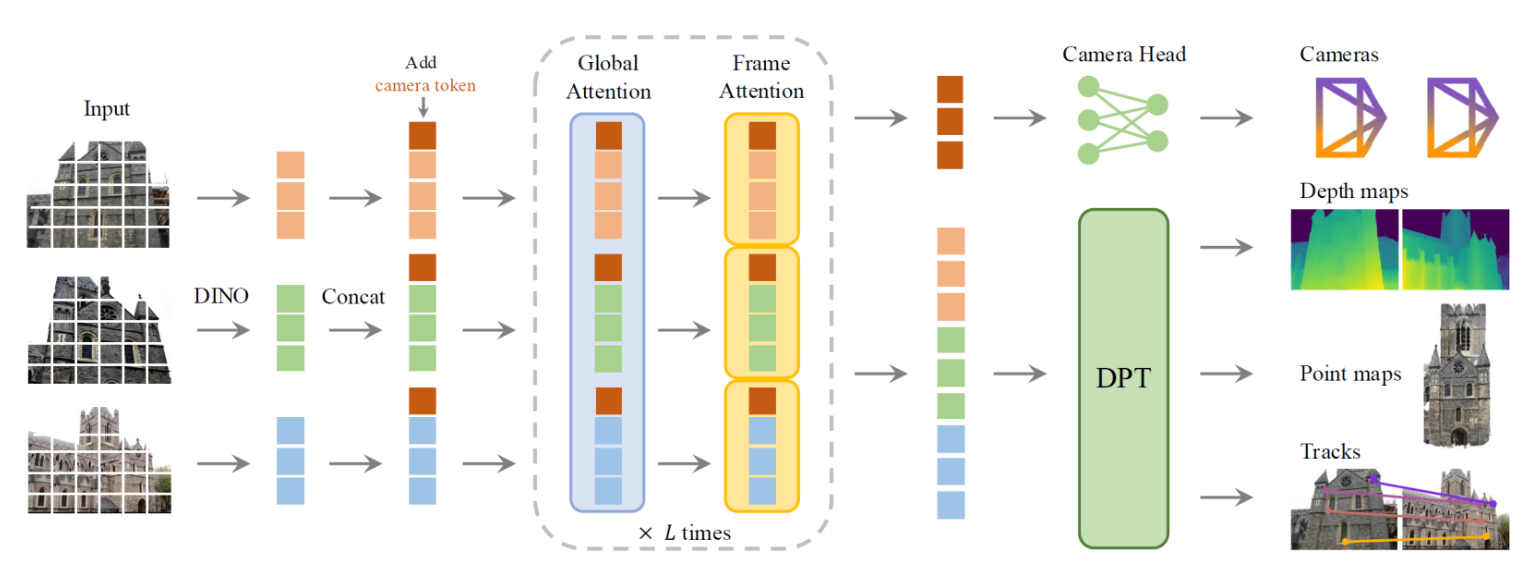
VGGT — Visual Geometry Grounded Transformer

• Feed-forward neural network that takes in input 1 or multiple images and can infer (1) camera parameters, (2) depth and point maps and (3) 3D point tracks in one single pass.
• Alternating attention: attention alternates on each frame and globally, since one layer looks at the big picture and one looks closely to the current image.
• Trained using many existing open-source datasets. Faster and more efficient than previous methods.

VGGT SLAM 2.0

• Create a new factor graph design while still addressing the reconstruction ambiguity of VGGT given unknown camera intrinsics
• Exploit VGGT attention layers for false positive matches rejection and for completing more loop closures
• Deployable onboard a ground robot using a Jetson Thor with real-time performance while running online — which is definitely impressive.

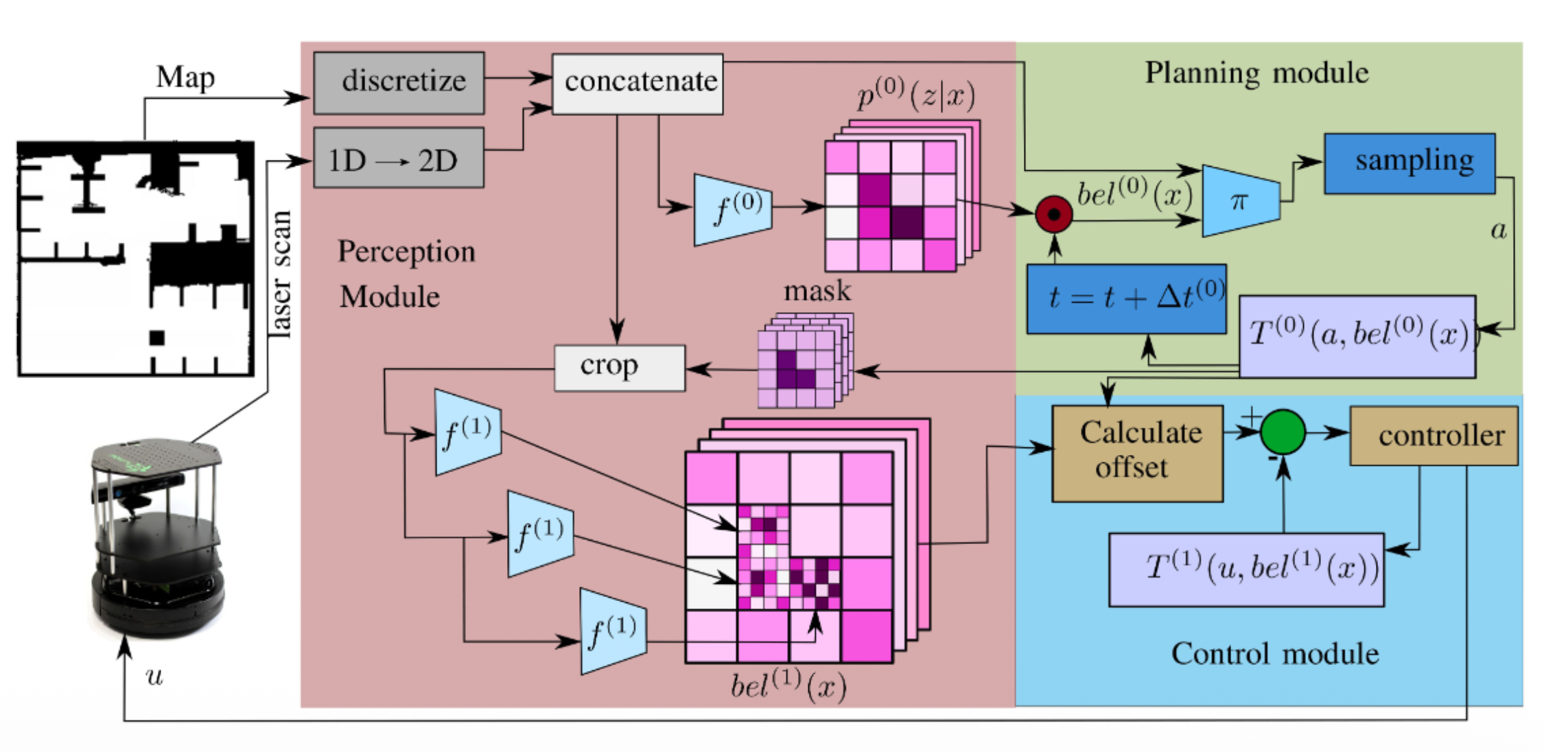
Deep active localization: Active localization consists of generating robot actions to maximally disambiguate its pose within a reference map.

• The system is composed of two learned modules: a convolutional neural network for perception, and a deep reinforcement learned planning module.