Transformers in depth and time

The mean-field particle perspective

We started with a small recap on Neural ODEs. The concept is basically an extension of the mathematics covered in Normalizing Flows and Change-of-Variable Formula.

The goal is to plan a path (via K and $b$) such that the initial data can be linearly separated. It happened automatically in NNs and Neural ODEs show that. It’s called gradient flow. See Deep Neural Networks Motivated by Partial Differential Equations, J Mathematical Imaging and Vision, 2019. Also Neural Ordinary Differential Equations, Neurips, 2018.

---

From Discrete Layers to Continuous Dynamics

The idea is that a deep Transformer with many layers can be viewed as a continuous-time dynamical system. We treat the layer index $k$ as a time variable $t$, and each token ${\mathbf{X}}_i$ is a particle evolving over time. The standard self-attention update is:

$$A_{ij}=\frac{\text{exp}({\mathbf{X}}_i\cdot D{\mathbf{X}}_j)}{{\sum }_{k=1}^N\text{exp}({\mathbf{X}}_i\cdot D{\mathbf{X}}_k)}$$

where $D=Q\cdot K$ is the product of query and key matrices, computes how much token $j$ should influence token $i$. The softmax ensures the sum is 1 so $A_{ij}$ is a proper probability over all tokens.

The full self-attention layer (including the residual connection from before) is:

$$A(X)=[{\mathbf{X}}_i+\sum _{j=1}^N{A}_{ij}V{\mathbf{X}}_j{]}_{i=1}^N$$

Each token ${\mathbf{X}}_i$ is updated by adding a weighted mixture of all other tokens, transformed by the value matrix $V$. We assume $V=D$ or $V=-D$ (which keeps the gradient flow structure — meaning the system minimizes a well-defined energy).

---

Layer Normalization

RMSNorm is moving the current distribution to a sphere. It constraints all tokens to have unit norm, up to a learned rescaling.

$$\text{RMSNorm}(x{)}_i=g_i\frac{x_i}{||x|{|}_2}$$

• $g[i{]}_{i=1}^n$ are learned parameters
• The projection $\prod (x)=\frac{x}{||x|{|}_2}$ restricts dynamics to the sphere $S^{n-1}$.

So after each attention step, we project back to the sphere:

$${\mathbf{X}}_i^{k+1}=\prod ({\mathbf{X}}_i^k+\sum _{j=1}^N{A}_{ij}(t)V{\mathbf{X}}_j^k(t)),i=1,\dots ,Nk=1,\dots ,K$$

This means: at every layer, each token moves in the direction of the weighted average of all other tokens, then gets snapped back to the unit sphere. K plays with depth (how many layers = how long time runs).

---

Discrete $\to$ Continuous Time

Now we go from discrete layers to a true ODE. Call $t$ an artificial “time” and $\Delta t$ a small step. Moving from layer $t$ to $t+\Delta t$:

$${\mathbf{X}}_i(t+\Delta t)=\prod ({\mathbf{X}}_i(t)+\Delta t\sum _{j=1}^N{A}_{ij}(t)V{\mathbf{X}}_j(t))$$

This looks exactly like Euler’s method. Now subtract ${\mathbf{X}}_i(t)$ and divide by $\Delta t$, then take $\Delta t\to 0$:

$$\frac{{\mathbf{X}}_i(t+\Delta t)-{\mathbf{X}}_i(t)}{\Delta t}\to ⟨{\nabla }_x\prod ({\mathbf{X}}_i(t)),\sum _{j=1}^N{A}_{ij}(t)V{\mathbf{X}}_j(t)⟩$$

The inner product $⟨\cdot ,\cdot ⟩$ here means: project the attention-weighted sum onto the tangent plane of the sphere at ${\mathbf{X}}_i(t)$. In the continuous limit $\Delta t\to 0$, it becomes a Neural ODE.

So the Transformer is literally an ODE solver for token dynamics on a sphere. “Going to infinite time” means running many layers until the dynamics converge.

---

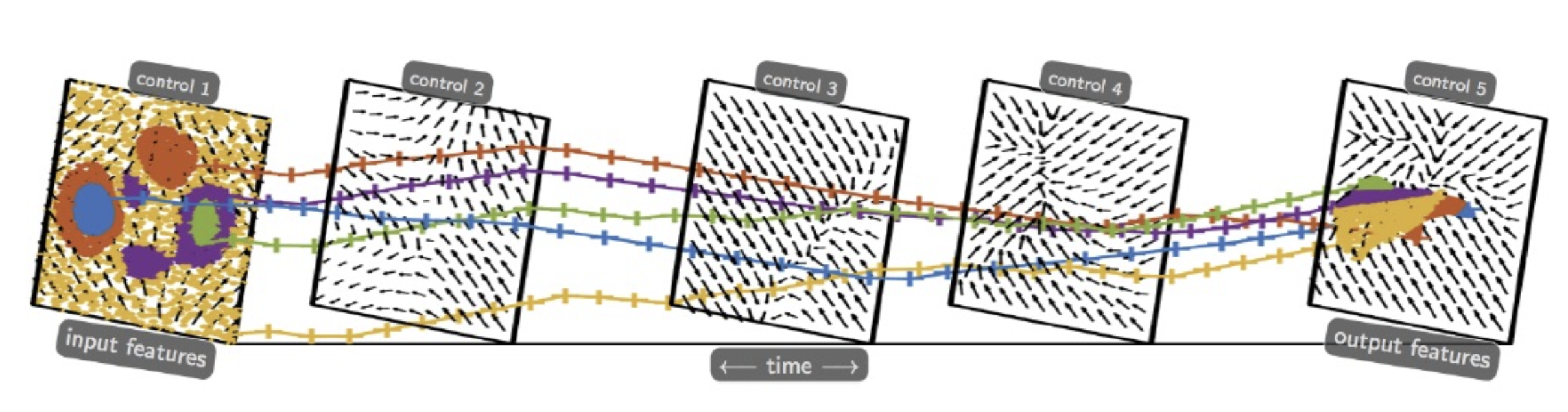
From Particles to a Distribution

Instead of tracking each of the $N$ tokens individually, we can describe them collectively as a probability distribution. The empirical measure is:

$${\mu }_t=\frac{1}{N}\sum _{i=1}^N{\delta }_{{\mathbf{X}}_i(t)}$$

So basically it’s just a sum of Dirac point masses — one at each token’s location at time $t$. The sum ${\sum }_{j=1}^N{A}_{ij}(t)V{\mathbf{X}}_j(t)$ is then an integral w.r.t. ${\mu }_t$. For a generic measure $\mu$ on the sphere, the velocity field each token experiences is: something too terrible for the normal eye to see…

$$V[\mu ](x)=\frac{P_x^{\perp }!\left({\int }_{\mathcal{S}}{e}^{x\cdot Dy}{V}_y;\mathrm{d}\mu (y)\right)}{{\int }_{\mathcal{S}}{e}^{x\cdot Dy};\mathrm{d}\mu (y)}$$

It’s the continuous version of softmax attention — instead of a sum over $N$ tokens, it’s an integral over the full distribution $\mu$.

Once we have a velocity field $V[{\mu }_t]$ that tells each token how to move, the distribution ${\mu }_t$ itself evolves according to the continuity equation (also called the transport equation):

$${\partial }_t{\mu }_t+div(V[{\mu }_t]{\mu }_t)=0$$

If you take the entries of the gradient and sum them up, you get the diversion $div$. Here comes the nice idea of the trace of the Jacobian Matrix from Flow Matching. This is how the Transformer comes to its answer. ufffff…

In other words: if probability mass is flowing with velocity field $V$, this equation says “mass is conserved” — whatever flows in equals what flows out. The $div$ (divergence) is the sum of partial derivatives of $V$ in all directions — it measures whether the flow is compressing or expanding at each point. The Transformer arrives at its final output distribution by solving this PDE.

---

Interaction Energy and Gradient Flow

The continuity equation is a mean-field PDE. There’s also the energy it dissipates:

$$\mathcal{E}(\mu )=\frac{1}{2}{\int }_{\mathcal{S}}{\int }_{\mathcal{S}}{e}^{x\cdot Dy}\mathrm{d}\mu (x)\mathrm{d}\mu (y)$$

This interaction energy measures how “aligned” all token pairs are (via the kernel $e^{x\cdot Dy}$, which is large when $x$ and $Dy$ point in similar directions). The dynamics monotonically increase $\mathcal{E}$ along trajectories — tokens are being pushed toward mutual alignment. This is a gradient flow with respect to a modified Wasserstein (optimal transport) distance. Optimal transport of token distributions directly links to Flow Matching and Diffusion models.

---

Rank Collapse

The picture below is what rank collapse or mode collapse looks like in Transformers. And it can happen very easily apparently. So the eigenvalues of $D$ provide concrete explainability of issues like this (rank collapse). If $D$ changes in time, then we have Neural PDEs.

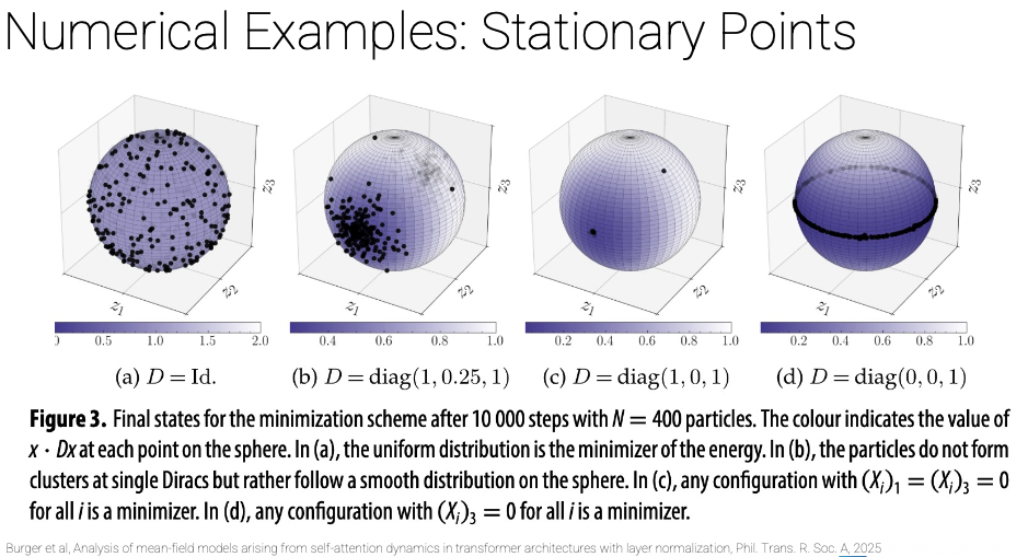
The stationary states of the dynamics depend entirely on the eigenvalues of $D$

• $D=Id$ (all eigenvalues equal 1): tokens spread uniformly on the sphere — no collapse.

• $D=diag(1,0.25,1)$: tokens cluster but don’t collapse to a single point.
• $D=diag(1,0,1)$: any configuration with the 1st and 3rd coordinates zero is a minimizer — collapse onto a great circle.
• $D=diag(0,0,1)$: full rank collapse — all tokens collapse to a ring in a single direction.

Rank collapse is when all tokens converge to the same (or a low-dimensional) representation, destroying the diversity of information. It’s the Transformer analogue of Mode Collapse in GANs. The eigenvalues of $D$ directly predict when and how this happens — zero eigenvalues in $D$ are the danger signal. If $D$ changes over time, we get Neural PDEs as a natural extension.

Final pipeline

• tokens are particles on a sphere $\to$ attention is a velocity field $\to$ running layers is solving an ODE $\to$ in the limit we get a PDE for the distribution $\to$ the eigenvalues of $D$ explain why collapse happens.

---

Learning Paradigms: Supervised, Unsupervised, Self-supervised

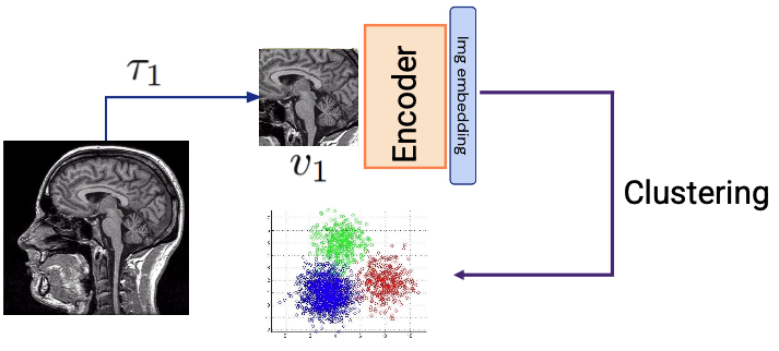
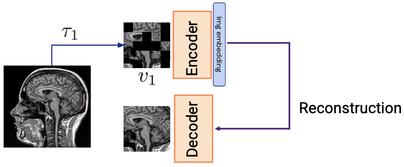
With Un-supervised learning we apply SVD and PCA to see the clusters that form in the data (cats that have similar faces sit together etc). One application is reconstruction: mask a patch of an image, encode the rest, decode to fill it back in. The reconstruction error acts as a self-generated training signal — but note, these models are not trained to be good at reconstruction as a final task; reconstruction is just the learning signal.

Self-supervised learning(SSL) is done through similarity or dissimilarity. You look at a patch for two different POVs (features) and compute how similar they are ⇒ there’s learning involved.

Consistent View Alignment

Take the same image and create two different augmented views (crops, flips): $v_1={\tau }_1(x)$ and $v_2={\tau }_2(x)$.

Compute their embeddings and train the model so representations of the same image are similar, and representations of different images are dissimilar. This gives me the (Dis-)Similarity signal.

The difference from unsupervised: in unsupervised you find structure that already exists (PCA clusters); in SSL you define a task (are these two views of the same image?) and the network learns features to solve it. Distillation (student-teacher) falls here: the teacher generates supervision signals for the student without human labels.

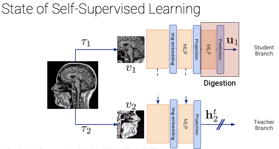
• First layer is on (dis)-similarity and feature extraction. This is the shared backbone (both student and teacher have it, with shared weights via the dashed arrows).
• Second layer is for “Disentanglement” of the learnt representations — the projection head separates the representation into independent factors (e.g. “shape”, “texture”, “position” become separate dimensions rather than entangled).
• Third layer is for “Digestion” (Prediction head, student only) — this is the extra MLP that only the student has. Its job is to predict the teacher’s representation $h_2^t$​ from the student’s projection $u_1$​. This is the clever trick that prevents collapse: the asymmetry between student (with prediction head) and teacher (without) means the network can’t trivially output the same constant for everything and still minimise the loss.

Why doesn't this collapse to all-constant features?

Because the teacher’s weights are an exponential moving average of the studen’t weights — so the target is always slightly “ahead”.

Self-supervised learning allows us to see what the heads are learning.

Golden rules of Self-supervised learning:

1. Don’t let your features collapse (make it stable) through contrastive loss (CLIP), teacher-student asymmetry (DINO).
2. Don’t make your features random. The similarity signal enforces this: two views of the same image must produce similar features, so the network is forced to learn something meaningful about the content.

Foundation Model

Anything that gives you meaningful re-usable features.