Single Image Depth Estimation (SIDE)

Why SIDE?

If you have no stereo camera available, and only a monocular camera; then you should apply SIDE.

Scenarios include:

• Dark / artificial-light environments — moving the camera changes the illumination, breaking structured-light or stereo assumptions.
• Highly dynamic scenes — the scene changes between frames t and t+1, invalidating multi-frame geometry.

Applications include indoor/outdoor robot navigation, obstacle avoidance, and autonomous driving.

Depth estimation means computing the distance from the camera to points in the scene. The single-image variant — often called SIDE — predicts a full depth map $D=f_{\theta }(I)$ from one RGB frame using a learned model. The key difference from stereo is that there is no geometric baseline to exploit — everything must be inferred from appearance alone.

How depth estimation works for humans

1. Occlusion — a partially covered object is perceived as farther away.
2. Perspective / texture gradient — same object looks smaller as distance grows; texture becomes denser.
3. Height cue — objects closer to the horizon line appear farther (vanishing point).
4. Shading & shadows — cast shadows give depth ordering between objects.
5. Atmospheric cue — objects get blurry and bluish as distance increases.

These cues reappear in the design of loss functions and model architectures below.

Traditional Methods

Saxena et al. (2006) — Make3D — was the first successful absolute-depth estimator from a single image using Markov Random Field.

• Log-space prediction: smaller depths can be more accurate, bigger depths are less accurate. Log compresses the range uniformly so it’s more tolerant with bigger depths.
• Global context: known-size objects (cars, people) can provide us cues to estimate the scale of the scene
• Relative depth error: subtracting the mean from both estimated and ground truth depth in log space removes scene-level scale ambiguity. Order of the depth of pixels instead of absolute depth (m)
• Markov Random Field (MRF): neighboring patches should have similar depth. Three sets of parameters: absolute depth, its uncertainty, and the smoothing strength.

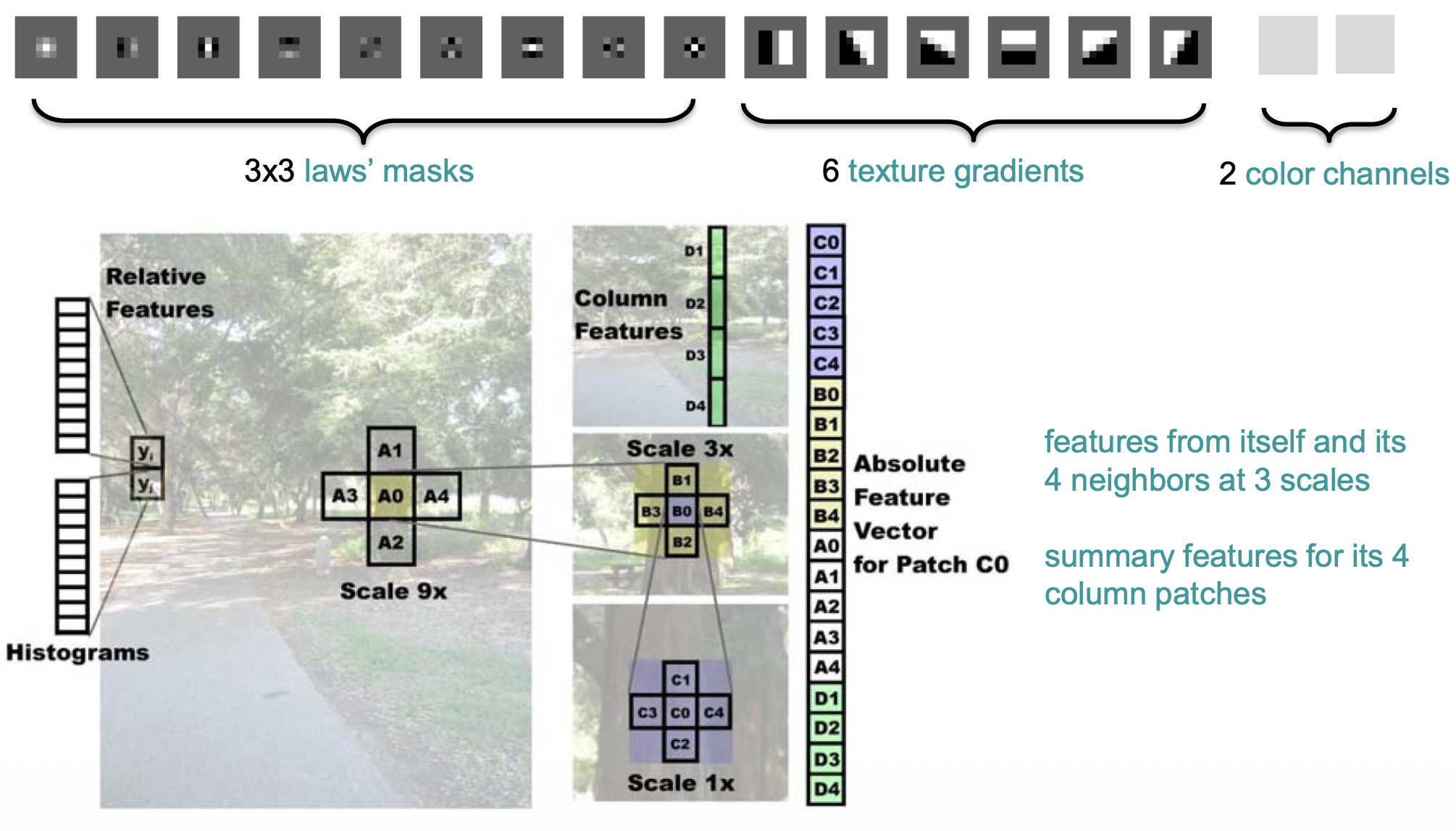
Above is the feature extraction diagram. For each patch (say C0 at Scale $1\times$), you don’t just look at the patch itself — you look at it at 3 different scales ($1\times ,3\times ,9\times$) and at its 4 spatial neighbors (up/down/left/right) at each scale.

The idea is: for each patch in the image, build a new vector that the MRF can use to predict its depth.

• $3\times 3$ Laws’ masks: small convolutional filters that capture texture (edges, spots, ripples).
• $6$ texture gradients: how the texture changes across the patch (directional gradient filters)
• 2 color channels: basic color information

Deep-Learning Approaches

All DL approaches share the same input/output structure: RGB image in, per-pixel depth map out. The challenge is that this is a one-to-many mapping, as many 3D layouts produce the same or nearly identical 2D image.

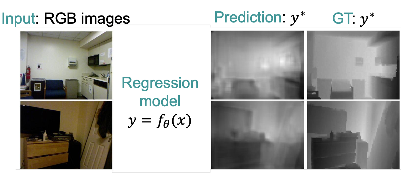
1. Regression

Direct pixelwise prediction with a squared-error loss:

$$L(y,y^{\ast })=\frac{1}{n}\sum _i(y_i-y_i^{\ast }{)}^2$$

Eigen et al. (2014) introduced a two-scale network:

• Coarse branch: sees the whole image, captures global context and scale.
• Fine branch: processes local patches, conditioned on the coarse result.

Their scale-invariant loss:

$$loss=\frac{1}{n}\sum _i(log({\hat{d}}_i)-log(d_i){)}^2-\frac{\lambda }{n^2}(\sum _i(log({\hat{d}}_i)-log(d_i){)}^2$$

When $\lambda =1$ this equals the L2 norm; the second term makes it scale-invariant. Later work added residual connections, deconvolution layers, and hybrid L1/L2 losses (L1 for short ranges, L2 for longer).

To optimize the process, one can use additional cues like normal vector values (estimated surface) and semantic labels.

2. Classification

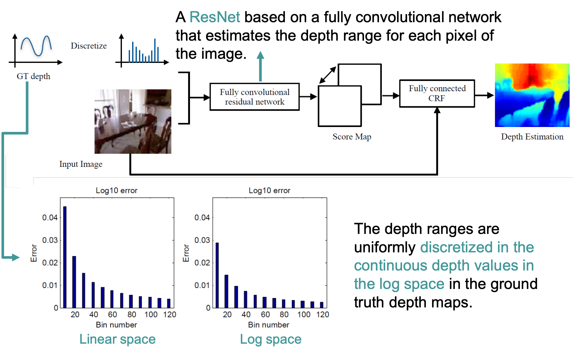
Cao et al. (2017) discretize the depth range into B bins in log space and treat each pixel as a classification problem, outputting a softmax probability distribution over bins.

• Depth ranges are uniformly discretized in log space — bins are narrower near the camera and wider far away.
• Training uses a cross-entropy loss weighted by an information-gain matrix H: depth ranges close to the ground truth are used to update the network’s weights.

$$loss=-\frac{1}{N}\sum _{i=1}^N\sum _{D=1}^{B}H(D_i^{GT},D)\log (P(D\mid z_i))$$

• Post-processing with a fully-connected CRF (Conditional Random Fields) refines per-pixel predictions using pairwise depth-consistency constraints between all pixel pairs. It works as a sort of refinement. The pairwise term penalizes assigning very different depth labels to pixels that should probably have similar depth

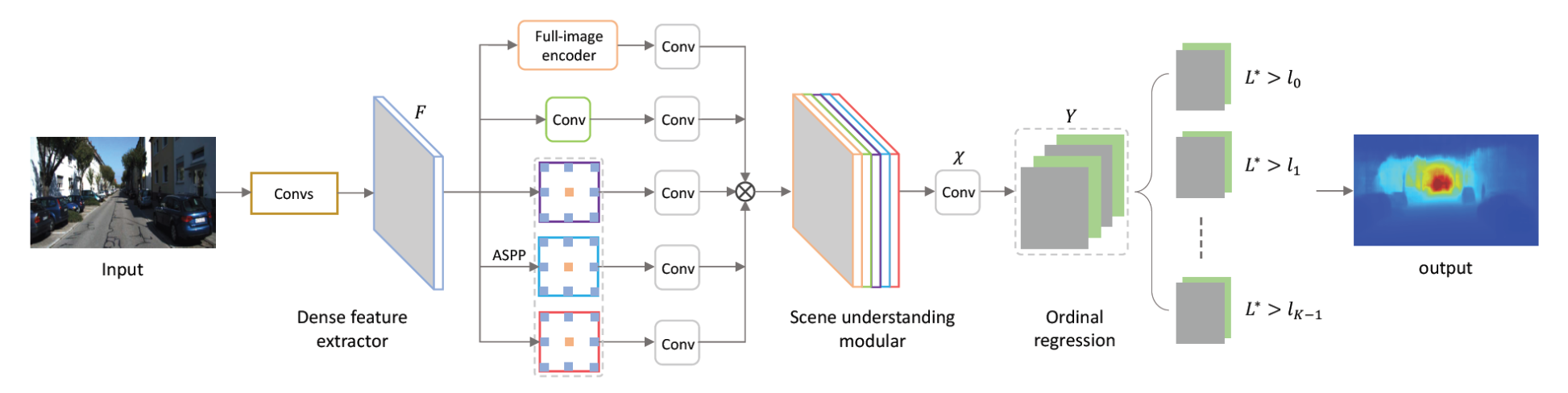
3. Ordinal Regression

Fu et al. (2018) frame depth as an ordinal problem: depth labels are ordered, so instead of one classification head, the network answers K binary questions “is this pixel’s depth greater than threshold t_k?”.

• i.e. the true depth of a pixel lies in the interval $l(w,h)\in \{0,1,2,\dots ,K-1\}$
• Inference: convert ordinal probabilities back to one depth

Spacing Increasing Discretization (SID)

• Depth prediction increases along with the underlying ground-truth depth
• Allow a relatively larger error when predicting a larger depth value to avoid over-strengthened influence of large depth values

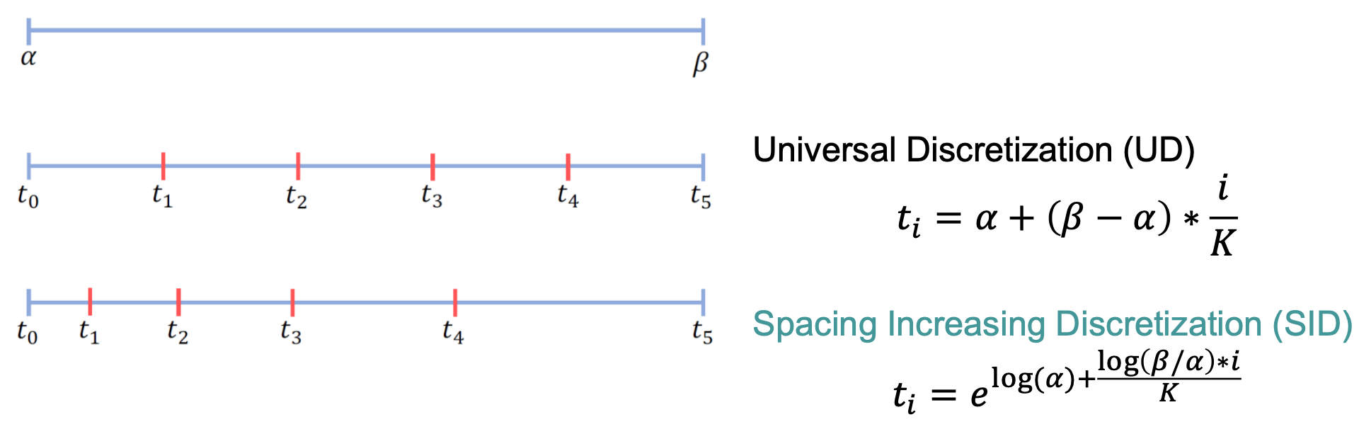
• UD spaces the thresholds linearly.
• SID spaces them logarithmically, giving finer resolution at close range and coarser at larger depths — matching real-world depths distribution.

The network uses Atrous Spatial Pyramid Pooling (ASPP) with dilated convolutions to extract multiscale context without increasing parameter count. Each of the K heads classifies all pixels simultaneously.

4. Multi-task Learning

Depth is estimated jointly with related tasks. The synergy improves results and robustness.

• Combinations of semantic and depth
• Combination of normal values and depth

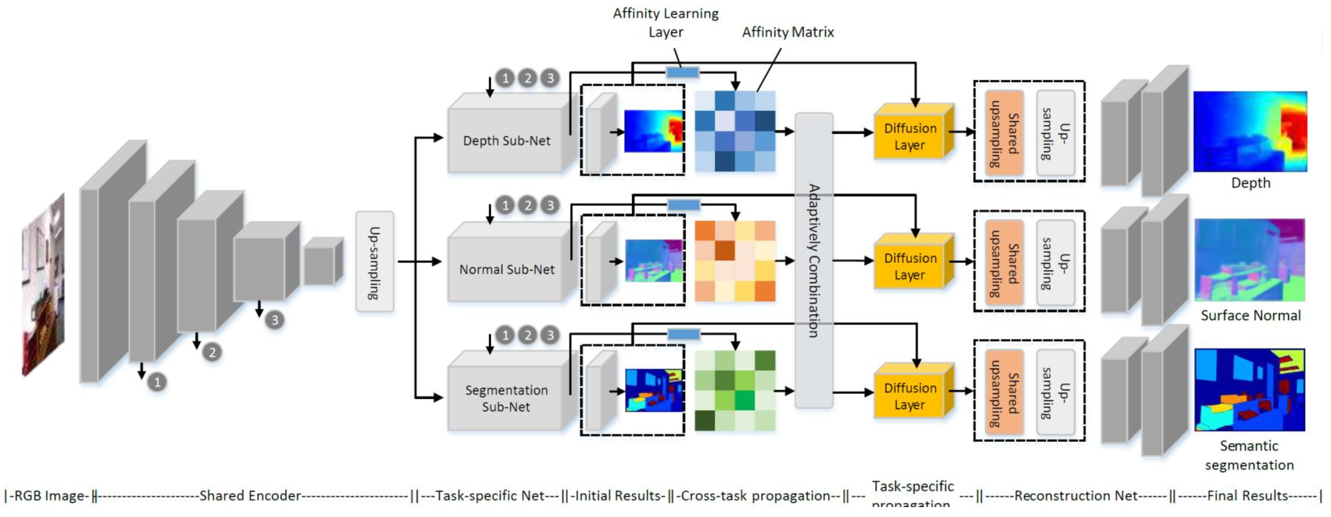
Pattern-Affinitive Propagation (PAP, CVPR 2019): similar pixel-pair relationship patterns appear across all three tasks. The model learns a shared affinity matrix and propagates it via diffusion layers.

5. Relative Depth

Generalisation across datasets is a core limitation — a model trained indoors fails outdoors. 

Relative depth sidesteps absolute-scale ambiguity by estimating pairwise orderings between (super)pixel regions rather than metric values. This allows training on diverse in-the-wild datasets without consistent depth scale.

$r_k$​ represents the ground-truth relative depth relationship between two sampled points or regions ($i_k$​ and $j_k$​) in an image. It acts as a label that dictates which loss function formula to apply based on the ordinal relationship of their depths:

• $r_k=+1$: Point $i_k$​ is closer to the camera than point $j_k$​ ($z_{i_k}<z_{j_k}$​​).
• $r_k=-1$: Point $i_k$​ is further away from the camera than point $j_k$​ ($z_{i_k}>z_{j_k}$​​).
• $rk=0$: Both points are at roughly the same depth ($z_{i_k}\approx z_{j_k}$​​).

Training Strategies

Supervised = Benchmarks

• basically datasets that provide the ground truth: KITTI, Sun RGB-D, $\dots$

Unsupervised / Self-supervised

Uses stereo image pairs or consecutive video frames. Two successive frames can act as a stereo pair. The core idea: warp the right image into the left viewpoint using the estimated depth, then minimize the photometric loss:

$$\widehat{I_L}=\text{warp}(I_R,D_L)=>Loss=|I_L-\widehat{I_L}|$$

Moving Objects Problem

Pixels on moving objects (e.g., a car) violate the static-scene assumption. The solution is to weight each pixel’s loss by a predicted belief produced by a separate mask network. Without known camera pose, a PoseNet must be run jointly — depth and pose are co-estimated, and depth maps must be scale-normalised.

Semi-supervised — Depth Anything V1 & V2

Foundation model approach. Gives relative depths (no metric values). A “teacher” model is trained on labelled data and assigns pseudo-labels to unlabelled images. Semantic priors from DINOv2 act as an auxiliary constraint. The student is trained on both. Perturbations are added to unlabelled inputs to enforce consistency. V2 improves the teacher and incorporates synthetic images.

Limitations

Current limitations include

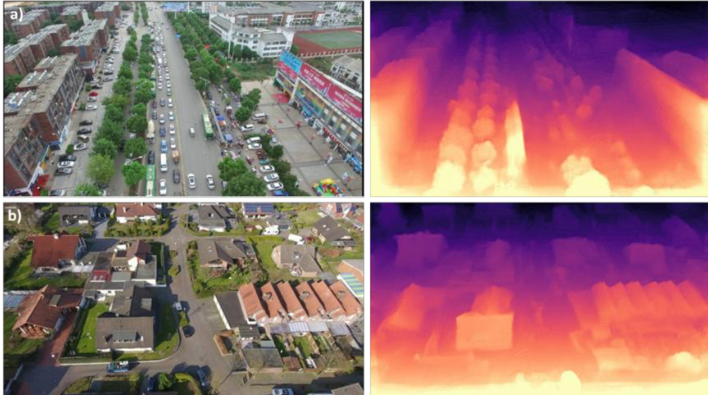
• Low transferability — appearance, camera intrinsics, object scale, and lighting all shift between datasets. A model trained on KITTI fails on aerial imagery.
• SIDE is still less accurate than stereo — stereo has an actual geometric disparity cue; single-image prediction is inherently ill-posed (many 3D scenes ⇒ same 2D image).
• Vertical position is the dominant cue (Dijk & Croon, ICCV 2019) — networks rely on where an object is in the image vertically, not just its size. Cropping the image differently fools the network. Objects must be connected to the ground plane to be detected as close.

Real-time deployment

Zhang et al. (CVPR 2023) showed SIDE can run in real-time on small onboard devices by combining CNNs and Transformers in a lightweight encoder-decoder.

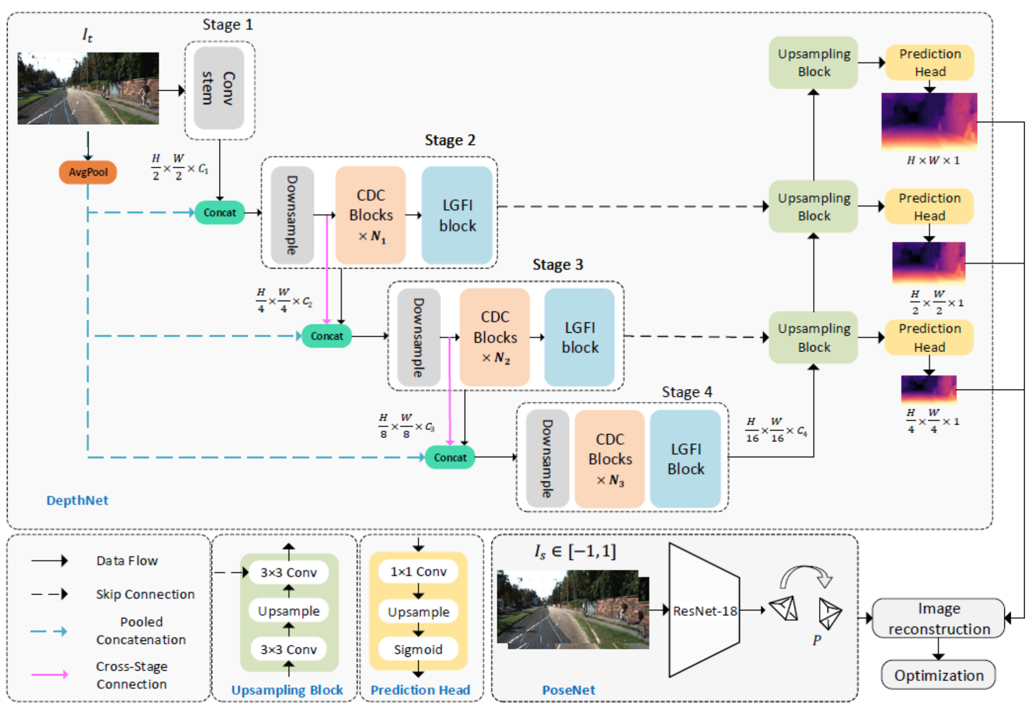
Lite-Mono Architecture

Four encoder stages downsample the input progressively. Each stage uses:

• CDC (Consecutive Dilated Convolutions) — multi-scale receptive fields without added parameters.
• LGFI (Local-Global Feature Interaction) — transformer-style attention block bridging local and global context.

Cross-stage skip connections (pooled concatenation) feed all encoder scales into three upsampling decoder heads at $H\times W,H/2\times W/2,$ and $H/4\times W/4$

• Knowledge distillation to reduce the “size” of the network. A follow-up work (Zhang et al., Drones 2024) used knowledge distillation to compress Lite-Mono further for nano-drones doing obstacle avoidance — the distilled network runs entirely onboard a tiny drone.

PoseNet (Kendall et al., ICCV 2015) is often covered alongside SIDE because pose and depth are co-estimated in self-supervised pipelines. It regresses 6-DOF camera pose directly from a single image.

Camera pose is given by translations ($x$) and rotations ($q$, in quaternion form). $\beta$ balances translation and rotation; it differs for indoor vs outdoor datasets. Also mentioned in Deep Learning SfM, SLAM, and VO.

$$Loss(I)=||\hat{x}-x|{|}_2+\beta ||\hat{q}-\frac{q}{||q||}|{|}_2$$