Fundamentals of parameter estimation - Part I

The fist exercise out of eight that I have to solve in the optimal estimation course.

In this case, I need to use the minimum risk (Bayes) estimators from The Estimation Paradigm (the static case) and also apply the knowledge from Introduction to Optimal Estimation and Dynamics.

Context

The measurement system

I need to estimate the depth of the water below a ship by using a ultrasonic depth gauge sensor. It is mounted on the bottom of the boat and presents a transmitter and a receiver which capture a tone burst transmitted downwards.

The principle is ToF (Time of Flight).

The ToF is proportional to the depth $x$. Let $c$ be the speed of sound in the water, then

$$x=\frac{c}{2}\cdot ToF$$

For clarity, we denote the true depth of the water with $x$ and the noisy measurement with $z$.

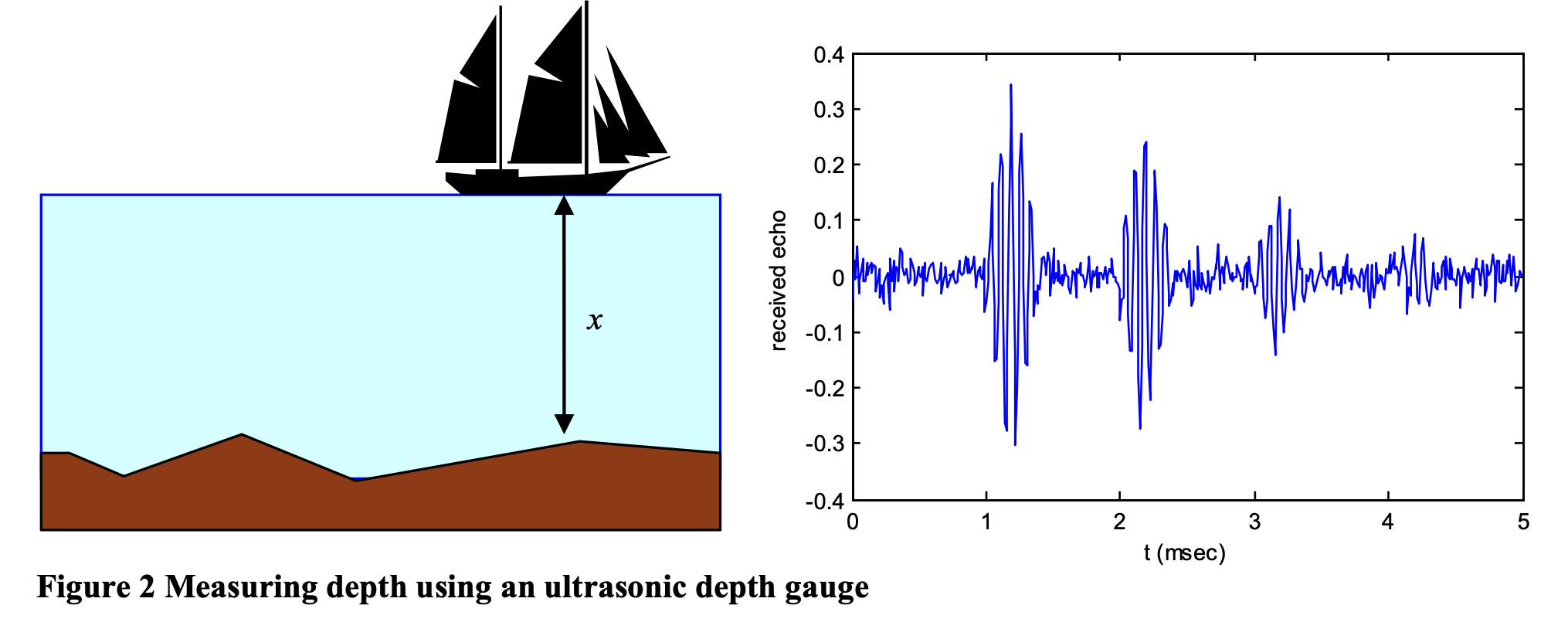
However, the measurement can be disturbed by multiple factors:

• Secondary echoes (Multipath Interference)
  • The echo may reflect at the bottom of the boat causing a second echo that arrives at $t=4x/c$. The second echo may cause a third echo, and so on. This makes the depth appear twice as deep ($2x$) than it actually is.
• Electronic noise
  • The measurement is contaminated by Gaussian noise with standard deviation $\sigma$. If we assume that $x$ is the real depth and $z$ is the result of our measurement, we can adopt the following Gaussian mixture model (Likelihood Function) for the conditional probability density of $z$

$$p(z\mid x)=P_0\frac{1}{\sigma \sqrt{2\pi }}\text{exp}(-\frac{(z-x{)}^2}{2{\sigma }^2})+P_1\frac{1}{\sigma \sqrt{2\pi }}\text{exp}(-\frac{(z-2x{)}^2}{2{\sigma }^2})$$

$P_1$ is the probability that the first echo is missed and replaced by the second echo. Obviously, $P_0$ is the probability that the first echo is correctly detected. $P_0+P_1=1$.

In simple words, electronic interference adds “jitter” to the measurement, represented by a standard deviation $\sigma$.

Prior Knowledge (Ground-Truth)

Based on the information from a nautical map, the shipper has some prior knowledge about the depth. The map indicates an interval of possible depths. This interval is considered to be softly bounded. Such prior knowledge can be modeled with a Generalized Normal Distribution.

$$p(x)=\frac{\beta }{2\alpha \Gamma \left(\frac{1}{\beta }\right)}\exp \left(-{\left(\frac{|x-\mu |}{\alpha }\right)}^{\beta }\right)$$

So, the captain gives the Prior Distribution $p(x)$. Instead of a standard bell curve, it uses a Generalized Normal Distribution, which allows for a “softly bounded” interval of likely depths using parameters $\alpha$ (scale), $\mu$ (mean), and $\beta$ (shape).

For example, if the depth interval is $[x_{min},x_{max}]$, then $\mu =\frac{1}{2}(x_{min}+x_{max})$ and $\alpha =\frac{1}{2}(x_{max}-x_{min})$

My case

For the current case, the following parameters are given:

• sensor system $p(z\mid x)$
  • $P_0=0.95$
  • $\sigma =0.1$
• prior knowledge $p(x)$
  • $x_{min}=1m$
  • $x_{max}=3m$
  • $\beta =20$

---

First Question: If we model $p(x)$ and $p(z\mid x)$ against $z$ for $x=1.5m$ and $x=2m$, what do these PDFs model?

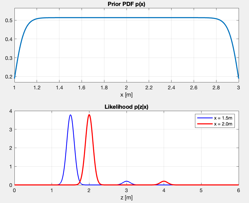
• The prior $p(x)$ shows my belief before even measuring. It’s nearly uniform between $x_{min}=1m$ and $x_{max}=3m$, meaning I consider all depth in that range roughly equally likely. Again, this one reflects the captain’s knowledge based on the nautical map.
• The Likelihood $p(z\mid x)$ tells me what measurement I should expect given the two true depths (blue with $x=1.5m$ and red with $x=2m$).
  • The blue PDF shows two peaks - one main peak at $z=1.5m$(correct echo, 95% probable), and a small peak at $z=3m$(secondary echo at 2x, 5% probable)
  • Same thing for the red PDF - main peak at $z=2m$ and small peak at $z=4m$.
• The peaks are sharp, showing the sensor is precise ($\sigma =0.1m$).

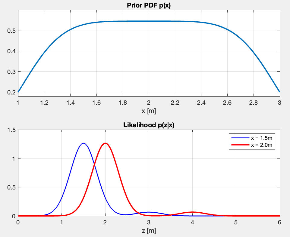
What happens if I modify $\sigma$? But $\beta$?

Modifying $\sigma$:

• The peak location stays the same, but the PDFs are more spreaded. As $\sigma$ >>, the noise gets larger ⇒ the measurement is less precise
• The integral under each peak stays the same
• But the probability of getting a measurement near a value changes. The peak heights change.
• With $\sigma =0.3$ (wider), there’s higher probability of measuring $z=1.7m$ when $x=1.5m$. With $\sigma =0.05$(narrower), that probability is much lower.

Modifying $\beta$:

• Changes which depths are considered more likely a priori
• As $\beta$ >>, I approach uniform distribution, meaning I assign all probabilities the same weight.
• In my current case, $\beta =20$ is good for “depth is somewhere between 1-3m, no strong preference”.

example for $\beta =5$ and $\sigma =0.3$

---

Second Question: Compute the PDFs regarding $p(z)$ and $p(x\mid z)$. Now we model these against $x$ for $z=3.1m$ and for $z=4m$.

What do they represent?

The evidence $p(z)$ is the total probability of observing a measurement $z$. It is calculated by integrating the likelihood over all possible true depths $x$.

$$p(z)={\int }_{\infty }^{\infty }p(z\mid x)p(x)dx$$

The posterior $p(x\mid z)$ represent my updated belief about the true depth $x$ after seeing measurement $z$. Per Bayes’ Theorem:

$$p(x\mid z)=\frac{p(z\mid x)p(x)}{p(z)}\propto p(z\mid x)p(x)$$

The marginal PDF $p(z)$ and the posterior PDF $p(x\mid z)$ look like this:

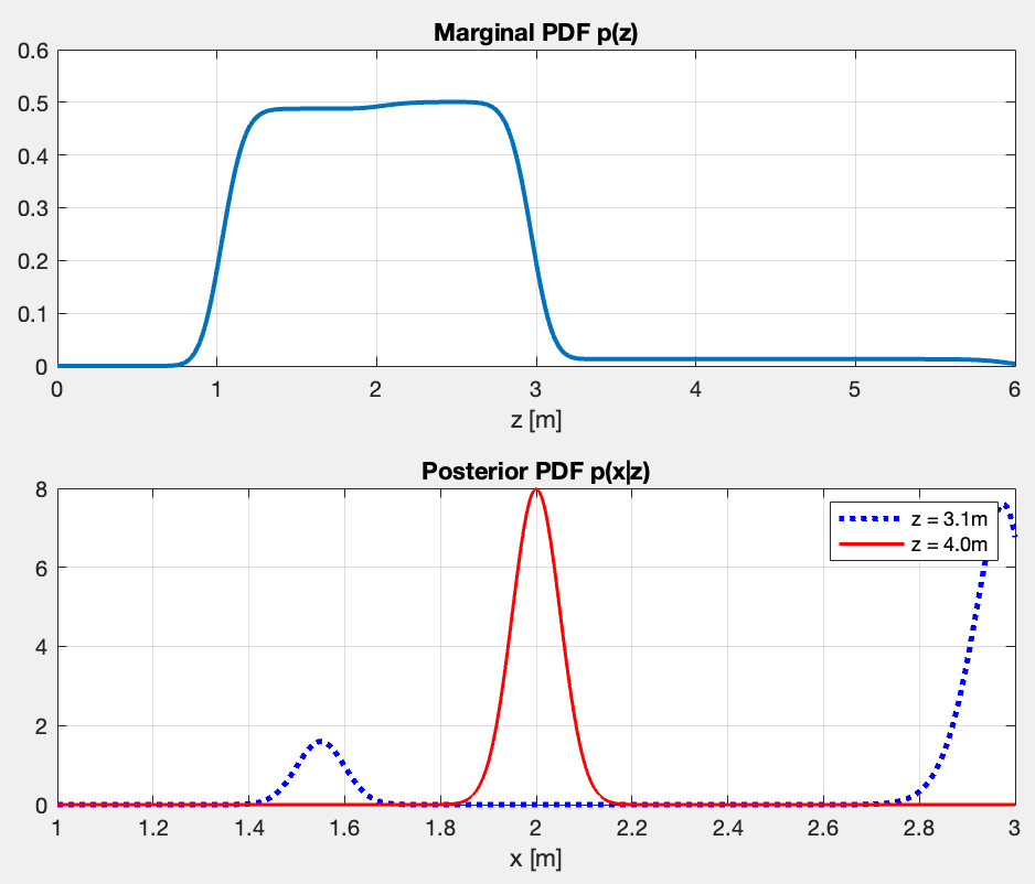
• The top plot $p(z)$ shows the two plateaus — the taller one for $z\in [1,3]$ corresponds to the $90\%$ chance of a direct reflection from the uniform prior $x\in [1,3]$. What follows is the $10\%$ plateau which corresponds to the echoes.
  • “What measurement are we likely to see?”
• The bottom plot $p(x\mid z)$ captures the two cases mentioned above.
  • “Given I measured $z$, what is the true depth $x$?”
  • For $z=4m$, a direct reflection is impossible since the maximum known depth is $3m$ (I know that from the prior). Therefore a measurement of $4m$ cannot possibly be a direct echo. The model infers it must be a double reflection which happens at $2x$, resulting in the distinct, confident peak at exactly $x=2.0m$ for $z=3.1m$.
  • In the case for $z=3.1m$ is ambiguous and presents two conflicting possibilities. It could be a double reflection, meaning the true depth is half of the measurement (the first small peak at $\sim x=1.55m$). Alternatively, it could be a direct reflection of a true depth very close to the $3m$ maximum, pushed up to $3.1m$ by sensor noise. Since direct reflections are highly probable, the model strongly leans toward this explanation, causing the massive spike at the $x=3.0m$ boundary.

---

Third Question: Create m-files that calculate:

• The MMSE estimator ${\hat{x}}_{\text{MMSE}}(z)$ for $z=3.1\text{m}$ and for $z=4\text{m}$.
  • Minimum Mean Square Error calculates the expected value, or the center of mass, of the posterior distribution. It minimizes the squared error of the estimate, meaning its position is influenced by all possible outcomes, including the small distant probabilities of secondary echoes.
  • ${\hat{x}}_{MMSE}=\int xp(x\mid z)dx$
• The MAP estimator ${\hat{x}}_{\text{MAP}}(z)$ for $z=3.1\text{m}$ and for $z=4\text{m}$.
  • Maximum A Posteriori maximizes the posterior distribution $p(x\mid z)$. It identifies the absolute highest peak of the combined probability, representing the single most likely depth when both the sensor measurement and the prior bounds are factored in.
  • ${\hat{x}}_{MAP}=\arg {\max }_{x}p(x\mid z)$
• The MMAE estimator ${\hat{x}}_{\text{MMAE}}(z)$ for $z=3.1\text{m}$ and for $z=4\text{m}$.
  • Minimum Mean Absolute Error calculates the median of the posterior distribution. It finds the exact depth that divides the total probability area perfectly in half, making it more robust against distant secondary peaks than the MMSE. (look more into this)
  • ${\hat{x}}_{MMAE}={\int }_{-\infty }^{x}p(x^{\prime }\mid z)d{x}^{\prime }=0.5$
    • In other words, minimize the expected absolute error $\mathbb{E}[|x-\hat{x}|\mid z]$. The solution is provably the median of the posterior, hence finding where the CDF(Cumulative Distribution Function) crosses 0.5.
• The ML estimator ${\hat{x}}_{\text{ML}}(z)$ for $z=3.1\text{m}$ and for $z=4\text{m}$.
  • Maximum Likelihood maximizes the the likelihood function $p(z\mid x)$. It strictly trusts the sensor data and finds the depth that makes the observed measurement most probable, completely ignoring the prior knowledge from the nautical map.
  • ${\hat{x}}_{ML}=\arg {\max }_{x}p(z|x)$

Can you explain the results, especially the ones for $z=3.1\text{m}$?

Results:

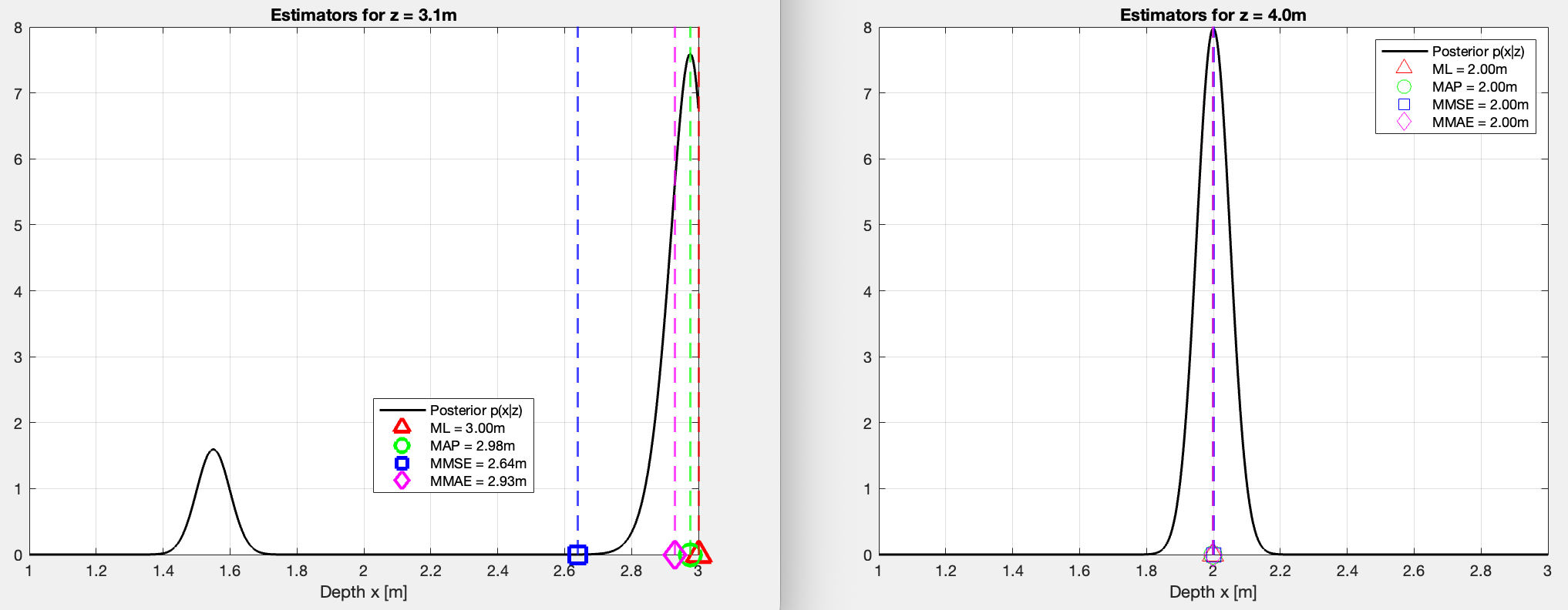
z=4m

All four estimators agree at $x=2m$. The posterior is unimodal so, naturally, all estimators converge because the prior eliminates any chance of a direct echo.

z=3.1m

In this case, the posterior is bimodal (two peaks which I explained earlier).

• The MMSE is the only one that’s pulled more to the left since it acts as a center of gravity. It does incline towards the correct answer, but in this case the value of 2.66 doesn’t make sense given the posterior.

• The MAP is the same as ML but multiplies the likelihood by the prior $p(x)$ first. The prior slightly penalizes $x=3.0$ since it’s near the boundary, nudging the peak marginally left to $x=2.98$. Very close to ML here because the likelihood peak dominates.

• The MMAE integrates the posterior from left to right until it has accumulated 50% of the total probability mass. The small left peak at $x=1.55$ contributes some mass, which means the $50\%$ point is reached slightly earlier than the MAP peak, pulling it to $2.93m$. Essentially asking “where is the middle of all the probability?”

  p(x|z)                        CDF
  |                              1|          ___
  |  /\      /\                   |         /
  | /  \    /  \                0.5|_ _ _ _/· · ·  ← median here
  |/    \  /    \                  |      /
  |      \/      \               0|_____/
  +-------------->x               +------------>x
  

• The ML looks at $p(z\mid x)$ and asks “for which x is this measurement most likely?”. It finds the peak of the likelihood. Since $z=3.1$ is just inside the prior boundary, the direct echo peak lands at $x\approx 3.0$. No prior involved at all.

---

Fourth+Fifth Question:

Calculate for each case in 3 the conditional risk. Compare and explain the results. Do that for any of the following cost functions:

• Quadratic cost function $(x-{\hat{x}}^2)$
• Absolute cost function $(|x-\hat{x}|)$
• Uniform cost function with $\Delta =0.5$. The definition of $\Delta$ is $C_{uni}(x\mid \hat{x})=1$ if $|x-\hat{x}|>\Delta$

The risks that are calculated may have a physical unit. Don’t forget to add them.

From The Estimation Paradigm, the risk is defined as the expected cost of an estimation error:

$$R(\hat{x}|z)=E_x[C(\hat{x}|x)|z]=\int C(\hat{x}|x)p(x|z)dx$$

z = 3.1m

Estimator	Quadratic (m²)	Absolute (m)	Uniform (-)
MMSE	0.3098	0.4435	0.9997
MAP	0.4100	0.3211	0.4838
MMAE	0.3819	0.3071	0.4732
ML	0.4258	0.3406	0.6333

z = 4.0m

Estimator	Quadratic (m²)	Absolute (m)	Uniform (-)
MMSE	0.0025	0.0399	0.3168
MAP	0.0025	0.0399	0.3267
MMAE	0.0025	0.0399	0.3267
ML	0.0025	0.0399	0.3267

• For $z=4.0m$ all estimators agree, so the risks are nearly identical across estimators for each cost function. The posterior distribution is unimodal, meaning there is only one logical explanation for the measurement.
• For $z=3.1m$ each estimator is lowest on its own cost function (MMSE lowest quadratic, MMAE lowest absolute, MAP lowest uniform) — exactly as the theory predicts.
• The uniform risk of MMSE at $z=3.1m$ is nearly $1.0$, meaning it almost always falls outside the $\Delta =0.05m$ window. Since the uniform cost function penalizes any estimate outside the 0.05m threshold, and there is virtually zero probability mass in that valley, the MMSE is almost guaranteed to incur the maximum penalty.