The Estimation Paradigm (the static case)

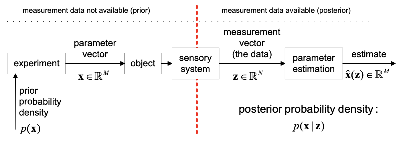
Estimation Paradigm

In the static case, we aim to estimate a fixed parameter vector $\mathbf{x}$ that does not change over time, based on a set of measurements $\mathbf{z}$.

• Physical Process: The source of the parameter $\mathbf{x}$.
• Sensory System: Maps the physical parameter $\mathbf{x}$ to a measurement vector $\mathbf{z}$.
• Estimator: A mathematical function $\hat{\mathbf{x}}(\mathbf{z})$ that produces an estimate of the true parameter based on the observed data.

Two Primary Design Approaches

A. Bayesian Approach

Uses a probabilistic model including prior knowledge. It minimizes a “probabilistic risk” based on a cost function.

• Requires: Prior PDF $p(x)$ and Likelihood $p(z|x)$.

B. Data Fitting Approach

Focuses on a measurement model and residuals (the difference between measured data and model-predicted data).

• Goal: Minimize an error norm of the residuals (e.g., Least Squares).

The Bayesian Framework

The Bayesian approach relies on Bayes’ Theorem to calculate the Posterior PDF, which combines prior beliefs with new evidence:

$$p(x|z)=\frac{p(z|x)p(x)}{\int p(z|x)p(x)dx}$$

The Estimation Process:

1. Define Prior PDF $p(x)$ (what we know before measuring).
2. Define Likelihood $p(z|x)$ (the sensor model).
3. Calculate Posterior PDF $p(x|z)=c\cdot p(x)p(z\mid x)$ (updated knowledge after measurement).
4. Minimize Conditional Risk $R(\hat{x}|z)$. Where ${\hat{x}}_{\text{MMSE}}=E[x\mid z]$ is the expected value of state $x$, given measurement $z$.

Risk is defined as the expected cost of an estimation error $\tilde{x}=\hat{x}-x$. The Bayes’ optimality criterion looks to minimize this integral.

$$R(\hat{x}|z)=E_x[C(\hat{x}|x)|z]=\int C(\hat{x}|x)p(x|z)dx$$ $${\hat{x}}_{\text{BAYES}}(z)=\arg \underset{\hat{x}}{\min }\int C(\hat{x}|x)p(x|z)dx$$

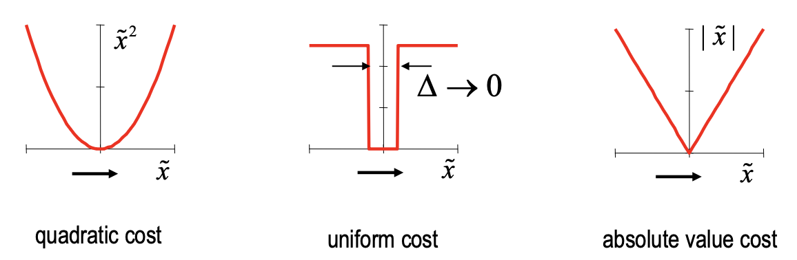
Where $C(\hat{x}|x)$ is the cost function in the scalar case (quadratic, uniform, absolute value), with

• $x$ the true parameter
• $\hat{x}$ the estimated parameter
• $\tilde{x}=\hat{x}-x$ the estimation error

The overall risk is over all $z$. I don’t know if I will have to use this form ever, but here it is:

$$R=E_z[R(\hat{x}(z)\mid z)]={\int }_{\infty }^{\infty }{E}_z[C(\hat{x}|x)|z]p(z)dz$$

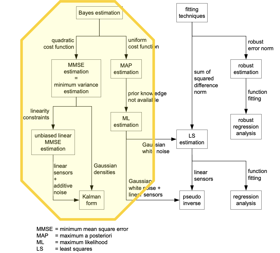
Bayes (minimum risk) estimators

• Quadratic cost $\to$ Conditional mean (MMSE)
  • You want to minimize squared error: $(x-\hat{x}{)}^2$
  • $\hat{x}(z)=E[x|z]$
• Absolute cost $\to$ Median (MMAE)
  • You want to minimize absolute error: $\left|x-\hat{x}\right|$
  • $\hat{x}(z)=\text{median}[p(x|z)]$
• Uniform cost $\to$ Mode (MAP)
  • You get penalized equally for any error, but zero cost if exactly correct
  • $\hat{x}(z)=\arg {\max }_{x}p(x|z)$

A quick example from Claude to help me understand these three concepts.

Imagine you’re trying to estimate someone’s age based on their appearance ($z$ = how they look). You have some uncertainty, so your belief is a probability distribution $p(\text{age}|\text{appearance})$.

Let’s say this distribution shows they’re likely between 25-35, with possibilities:

• 25 years: 10% chance
• 30 years: 70% chance
• 35 years: 20% chance

Now you must give ONE estimate. Which do you choose?

Quadratic cost (mean):

• If you’re wrong, the penalty grows with the square of your error
• Being off by 10 years is MUCH worse than being off by 5
• Best estimate: weighted average = 0.1×25 + 0.7×30 + 0.2×35 = 30.5 years

Absolute cost (median):

• If you’re wrong, penalty is just the absolute difference
• Being off by 10 is exactly twice as bad as being off by 5
• Best estimate: the middle value = 30 years

Uniform cost (mode):

• You either get it exactly right (no penalty) or wrong (same penalty regardless)
• Best estimate: most likely value = 30 years (the 70% one)

Different loss functions $\to$ different “best guess” from the same distribution.

Maximum Likelihood Estimation (MLE)

Also covered in MLE. Basically, we use this when no prior knowledge of $x$ is available (i.e. $x\sim N(0,{\sigma }^2)$ with $\sigma \to \infty$).

The MAP estimator in this case becomes the ML estimator:

$${\hat{x}}_{ML}(z)=\arg \underset{x}{\max }p(z|x)$$