Introduction to Optimal Estimation and Dynamics

The estimation paradigm involves taking a control signal (like engine thrust) and sensor data (such as range or speed) to determine the estimated properties of an object, such as its position, orientation, or velocity.

Key Components

• Dynamic & Kinematic Models: Mathematical equations that describe how a system changes over time.
• Process Noise: Unpredictable factors that cause a real track to deviate from a planned path. While noise itself cannot be predicted, the uncertainty it creates can be quantified.
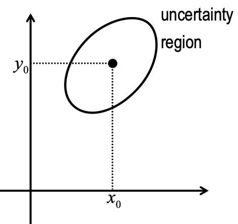
• Uncertainty Regions: Areas where an object is likely to be (e.g., a 91% probability region). These are mathematically represented by covariance matrices.

Therefore, an uncertain position is quantified by:

• the position of the uncertainty region: $\bar{\mathbf{x}}=\left[\begin{array}{c}{\mathbf{x}}_0\\ {\mathbf{y}}_0\end{array}\right]$ i.e. the expectation of the position,
• the size and shape of the region (the covariance matrix) $C_{\mathbf{x}}$.

Linearization through Taylor Series Expansion

From the nonlinear state equation:

$$\left[\begin{array}{c}x(i+1)\\ y(i+1)\end{array}\right]=\left[\begin{array}{c}x(i)\\ y(i)\end{array}\right]+T(V+\tilde{v}(i))\left[\begin{array}{c}\cos (\phi (i)+\tilde{\phi }(i))\\ \sin (\phi (i)+\tilde{\phi }(i))\end{array}\right]$$

If we apply 1st order Taylor Series, we get the linearized state equation:

$$\underset{\text{state}}{\underbrace{\left[\begin{array}{c}x(i+1)\\ y(i+1)\end{array}\right]}}=\left[\begin{array}{c}x(i)\\ y(i)\end{array}\right]+\underset{\text{control}}{\underbrace{TV(1-\frac{1}{2}{\sigma }_{\tilde{\phi }}^2)\left[\begin{array}{c}\cos \phi (i)\\ \sin \phi (i)\end{array}\right]}}+\underset{\text{process noise}}{\underbrace{\left[\begin{array}{c}{w}_1(i)\\ w_2(i)\end{array}\right]}}$$

We can define the linear state equation under this format:

$$\mathbf{x}(\mathbf{i}+1)=\mathbf{Fx}(\mathbf{i})+\mathbf{Lu}(\mathbf{i})+\mathbf{w}(\mathbf{i})$$

In the previous kinematic model, $\mathbf{F}=\mathbf{L}=\mathbf{I}$.

The propagation of uncertainty in time can be described mathematically by modelling how the covariance matrix changes in time.

$\mathbf{C}(\mathbf{i}+1)=\mathbf{FC}(\mathbf{i}){\mathbf{F}}^{\mathbf{T}}+{\mathbf{C}}_{\text{process noise}}$

where:

We define the statistical definition of process noise:

• $\mathbf{E}[\mathbf{w}(\mathbf{i})]=0$
• $\mathbf{E}[\mathbf{w}(\mathbf{i})\mathbf{w}(\mathbf{i}{)}^{\mathbf{T}}]={\mathbf{C}}_{\text{process noise}}$

And the statistical definition of initial conditions:

• $\mathbf{E}[\mathbf{x}(0)]=\bar{\mathbf{x}}(0)$
• $\mathbf{E}\left[\right(\mathbf{x}(0)-\bar{\mathbf{x}}(0)\left)\right(\mathbf{x}(0)-\bar{\mathbf{x}}(0){)}^{\mathbf{T}}]={\mathbf{C}}_{\text{init}}$

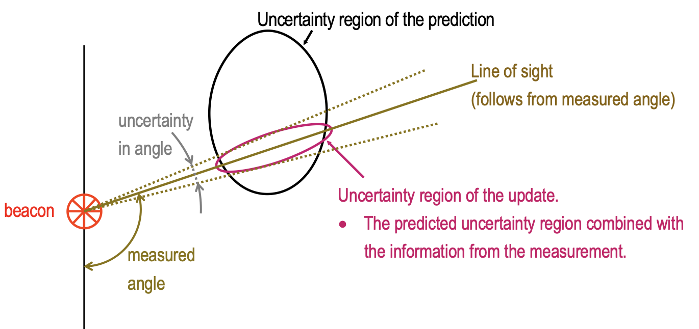
Updating = Prediction + Measurement

Basically, when the uncertainty of the prediction becomes too large, we perform measurements to calculate a new uncertainty region and recalculate the path.

Dead reckoning is simply estimating your future position given your current position and relative measurements.

• Here we use the first starting point as the reference position.
• If we make a loop along a coastline, we know the last point should be the initial point. Error comes from drift.

I guess we could call it a SLAM problem when we use landmarks (beacons) to anchor our positions.

Chapters from the book to look over for this part:

• 3 — parameter estimation (partly)
• 4 — state estimation
• 8 — state estimation in practice
• 9.3 — worked out example