Fundamentals of parameter estimation - Part II

This is the continuation to Fundamentals of parameter estimation - Part I. Exercise 2/8 from my optimal estimation course.

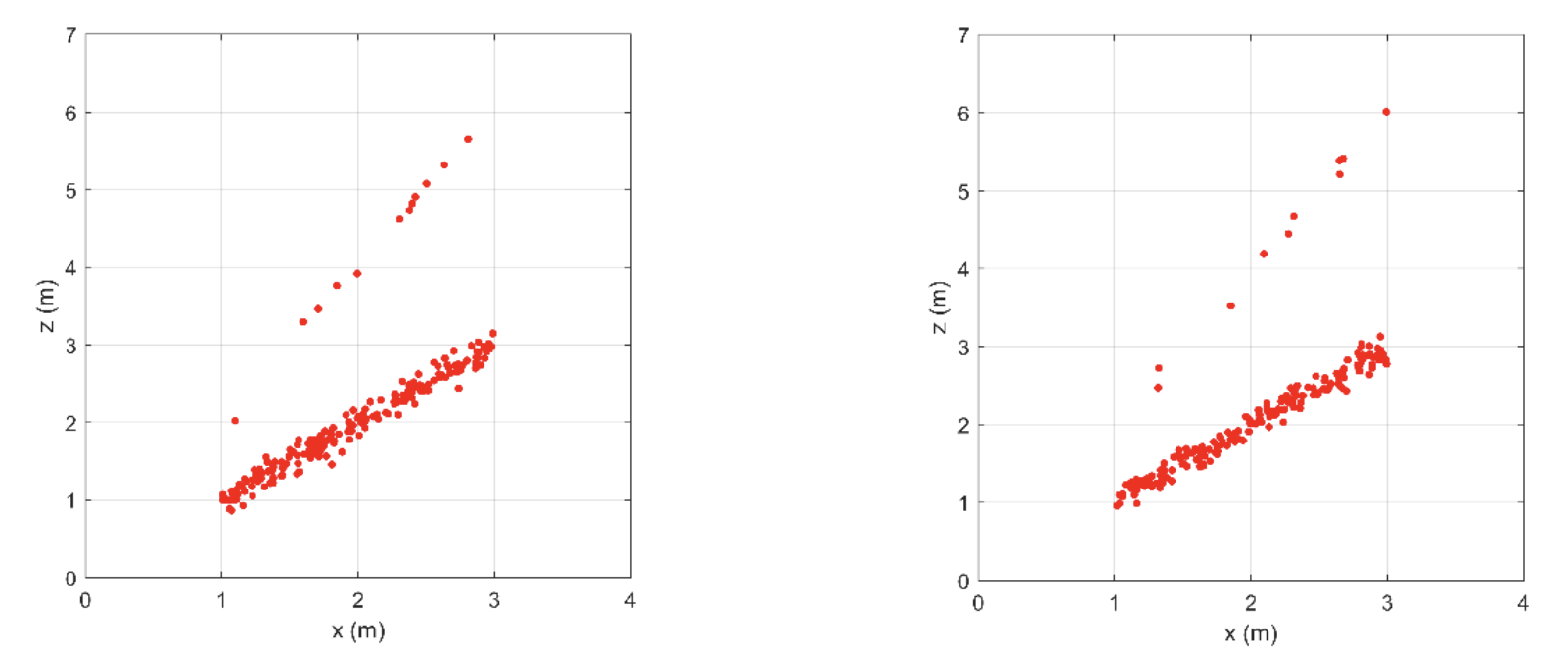
I need to reconsider the ultrasonic depth gauge discussed in Part 1. The Figure below shows two data sets that are obtained from the probabilistic model. Each data set contains 200 points $(x_n,z_n)$. The realizations are a-select and independent.

The goals, in the end, are:

• To design a linMMSE estimator and an unbiased linMMSE estimator using the first data set.
• To evaluate these estimators with respect to bias and variance using the second data set.

---

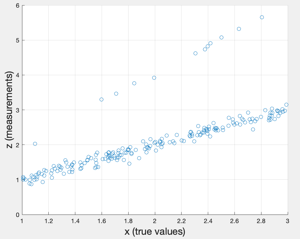
First topic: Create an xy-scatter diagram showing the true values $x_n$ against the measurements $z_n$.

---

Second topic: Design a linear MMSE estimator ${\hat{x}}_{lMMSE}(z)=\alpha z$, i.e. determine $\alpha$, using estimates of $\mathbb{E}[xz]$ and $\mathbb{E}[z^2]$ derived from the first data set.

$${\hat{M}}_{xz}=\frac{1}{N}\sum _{n=1}^N{x}_n{z}_n$$ $${\hat{M}}_{zz}=\frac{1}{N}\sum _{n=1}^N{z}_n^2$$

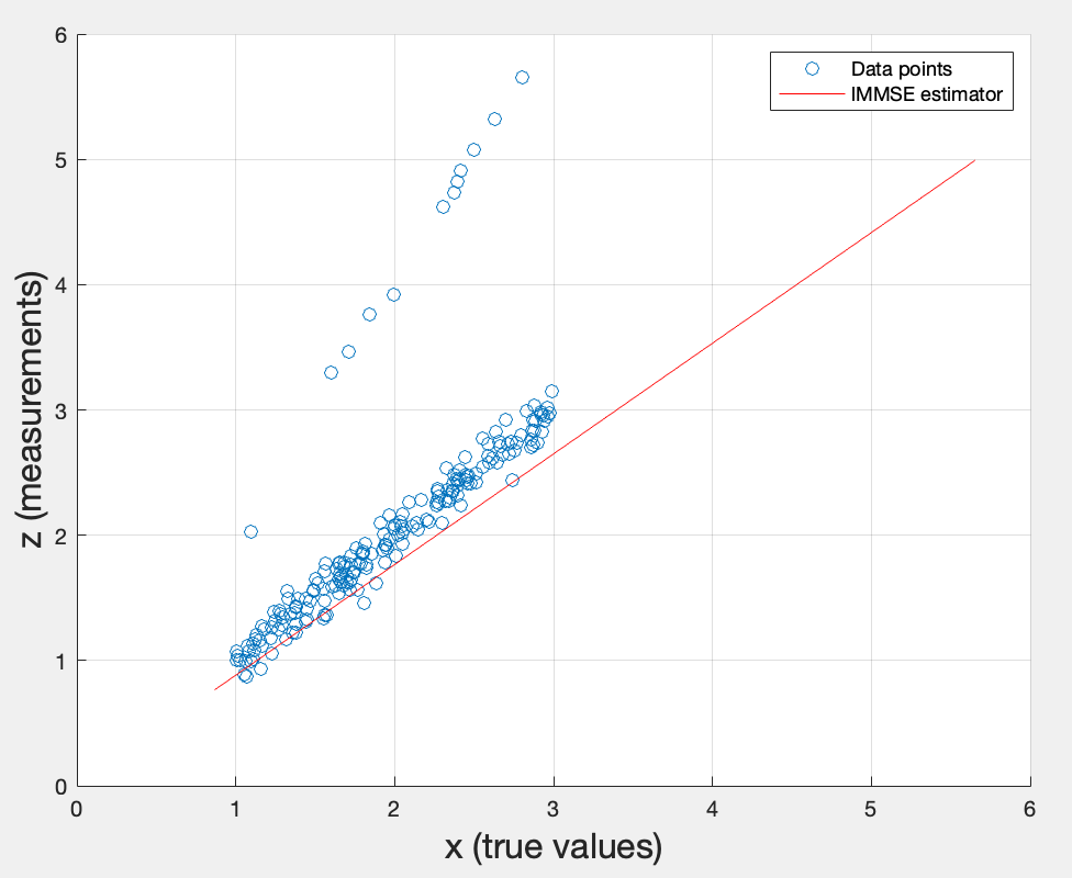
The line represents the best linear estimate of $x$ given $z$, passing through the origin (since there’s no offset $\beta$). It fits the main cluster of data reasonably well, but the outliers in the upper-left — those are likely the secondary echo measurements from the depth gauge model — pull the estimator slightly off.

To get derive the linear MMSE $\alpha$, I need to minimize the MSE cost function $J(\alpha )=\mathbb{E}[(x-\alpha z{)}^2]$. Now I take the derivative of $J$ w.r.t. $\alpha$ and set it to 0: $\frac{\partial J}{\partial \alpha }=-2\mathbb{E}[z(x-\alpha z)]=0$. Distributing the expectations gives $\mathbb{E}[xz]-\alpha \mathbb{E}[z^2]=0$, which gives $\alpha =\frac{\mathbb{E}[xz]}{\mathbb{E}[z^2]}$.

---

Third topic: Design the unbiased linear MMSE estimator ${\hat{x}}_{ulMMSE}(z)=\alpha z+\beta$, i.e. determine $\alpha$ and $\beta$, using estimates of $\mathbb{E}[x]$, $\mathbb{E}[z]$, $\text{Cov}[x,z]$, $Var[z]$ derived from the first data set.

According to the material, I can define the covariance between the two variables $x$ and $z$ like this:

$$\text{Cov}[x,z]=\mathbb{E}[(x-\bar{x})(z-\bar{z})]=>\widehat{\text{Cov}}[x,z]=\frac{1}{N-1}\sum _{n=1}^N(x_n-\hat{\bar{x}})(z_n-\hat{\bar{z}})$$

In MATLAB, $\text{cov}(x,z)$ returns a $2\times 2$ matrix: $\left[\begin{array}{ccc}\text{Var}(x)& & \text{Cov}(x,z)\\ \text{Cov}(z,x)& & \text{Var}(z)\end{array}\right]$. For that reason, it seems that I only need to select the second column from the first row.

From the provided equation, $\hat{x}(z)=\alpha z+\beta$, I can deduce that $\mathbb{E}[x]=\alpha \cdot \mathbb{E}[z]+\beta$.

Why? Because the unbiased linear MMSE estimator minimizes the MSE under the constraint that it is unbiased, meaning $\mathbb{E}[\hat{x}]=\mathbb{E}[x]$.

• Expanding with $\beta =\mathbb{E}[x]-\alpha \cdot \mathbb{E}[z]$, I go further into $\hat{x}=\alpha z+\mathbb{E}[x]-\alpha \mathbb{E}[z]$.
• Now I minimize the MSE cost function $J(\alpha )=\mathbb{E}[((x-\mathbb{E}[x])-\alpha (z-\mathbb{E}[z]){)}^2]$ by taking the derivative w.r.t. $\alpha$ and setting it to 0.
  • $\frac{\partial J}{\partial \alpha }=-2\mathbb{E}\left[\right(z-\mathbb{E}[z]\left)\right((x-\mathbb{E}[x])-\alpha (z-\mathbb{E}[z])\left)\right]=0$
  • It simplifies to $\mathbb{E}[(x-\mathbb{E}[x])(z-\mathbb{E}[z])]=\alpha \mathbb{E}[(z-\mathbb{E}[z]{)}^2]$
    • The left side is the definition of covariance, $\text{Cov}[x,z]$.
    • The right side is the definition of variance, $\text{Var}[z]$.
    • Dividing the two gives $\alpha =\frac{\text{Cov}[x,z]}{\text{Var}[z]}$

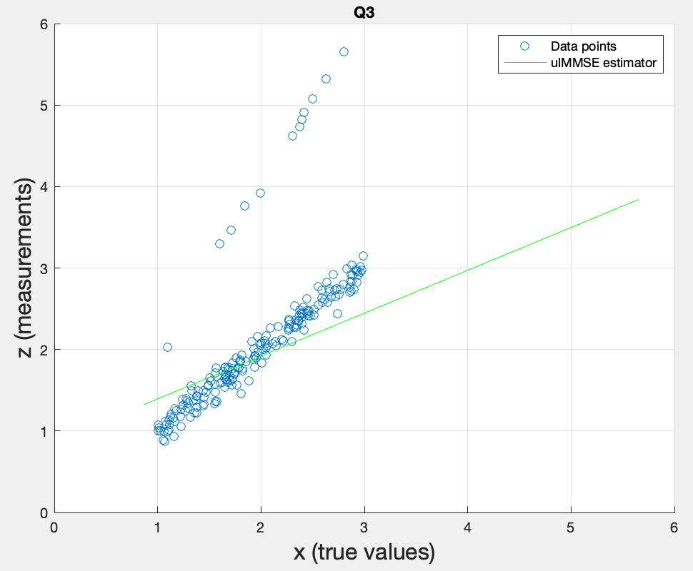
As a comparison, the ulMMSE line passes through the mean of the data $x,z$ (unlike the lMMSE which was forced through the origin), since the $\beta$ parameter allows the line to shift and pass directly through the mean value of the dataset. However, the outliers (secondary echoes) pull the overall mean slightly upward.

---

Fourth topic: Load the second data set. Apply the linear MMSE estimator that you have developed with the first set to the measurements $z_n$ from the second set. Determine the estimation errors ${\tilde{x}}_n={\hat{x}}_{\text{MMSE}}(z_n)-x_n$. Estimate the overall bias (mean of the estimation errors) and the variance of the errors.

Going back to the second topic, I know ${\hat{x}}_{lMMSE}(z)=\alpha z$. Therefore, I simply need to reuse the alpha from the second topic and apply it to this dataset.

Currently, I get a bias of -0.1488. It means the estimator systematically underestimates $x$ on average by ~0.15m. This is expected since lMMSE is forced through the origin and doesn’t account for the mean offset. The variance of 0.1993 reflects the spread of the errors.

---

Fifth topic: Do the same for the unbiased linear MMSE esimator.

	lMMSE (DS1)	lMMSE (DS2)	ulMMSE (DS1)	ulMMSE (DS2)
Bias	-0.1179	-0.1488	0.0000	-0.0501
Variance	0.2238	0.1993	0.1349	0.1372

• ulMMSE has near-zero bias on dataset 1 (0.0000) because it was designed with the unbiased constraint using that same dataset. On dataset 2 the bias is small (-0.0501) but not zero, since it’s a different sample.
• ulMMSE has lower variance (~0.135) compared to lMMSE (~0.2) on both datasets, meaning it’s also more precise.
• lMMSE has notable bias on both datasets (-0.1179 and -0.1488) because it’s forced through the origin, ignoring the mean offset.

---

Sixth topic: Why did we need to use a second dataset?

A second dataset is needed because evaluating bias and variance on the same data used to design the estimator would be overly optimistic — the estimator was literally fitted to that data. Dataset 2 gives an honest, independent evaluation of performance.