Efficient FoMos

Basically how Torch does it in the background. Optimizing the operations.

Alex first gave the example of transistor grids with 1000 nanometers $\times$ each square represents a 20 nanometer transistor. He also went on base-2 representation of numbers. With the Sign | Exponent | Significand and the precisions.

Single(32) / Half(16) / Double-point(64) precision float. The IEEE standard is half precision float (16 bits) (1 | 5 | 10). It allows values in the range of $\pm 65k$. However, it’s still very far from single precision, so we use Brain half.

• Negative numbers (two’s complement): flip all digits and add +1 to the end

Brain half precision float

Preserve 32-bit dynamic range, reduce fraction/significand precision.

So you can dynamically assign different number of bits to exponent and significand. We can represent more numbers, but with smaller precision. (1 | 8 | 7).

With Torch, it’s better to use Brain half precision float.

---

Hardware Improvements

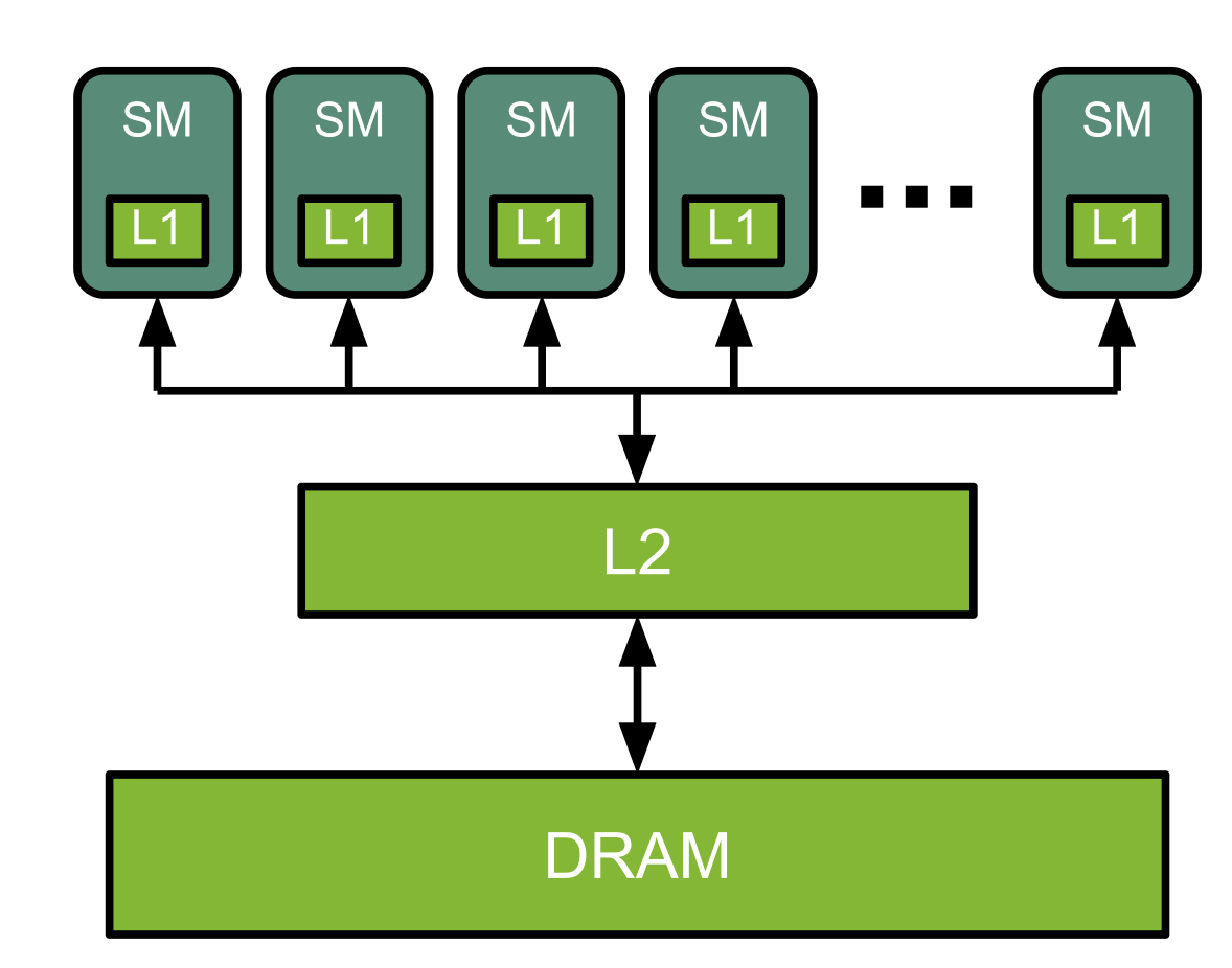
Here he started with the parallelism from NVIDIA Streaming Multiprocessors (SMs) where each cell is a computational unit in itself. I.e. the GPU.

• L1 cache (i.e., on-chip SRAM) — responsible for fast (low memory) computations
• L2 cache — shared memory accessible by all SMs - higher latency due to physically away from compute units.

DRAM (High Bandwidth Memory) not on the GPU die. Separate silicone connected with wires to the GPU die. This is basically the memory slots we have.

Attention in these terms:

• Read $Q,K$ from DRAM
  • Write $S=Q{K}^T$ back to DRAM
• Read $S$ to DRAM
  • Compute $A=softmax(S)$
  • Write it back to DRAM
• Read $A,V$ from DRAM
  • $O=AB$
  • Write O back to DRAM

Which is not very efficient, no? Because it’s sequential. That’s why we use L1 to parallelize it. But they are very small, only some kB. So we must optimize the process.

---

TILING

Let’s say we have 2 matrices and we want to do the dot product. In total we have $O(N^3)$ complexity. Tiling is about selecting smaller segments and computing those. See the slides, it’s quite smart.

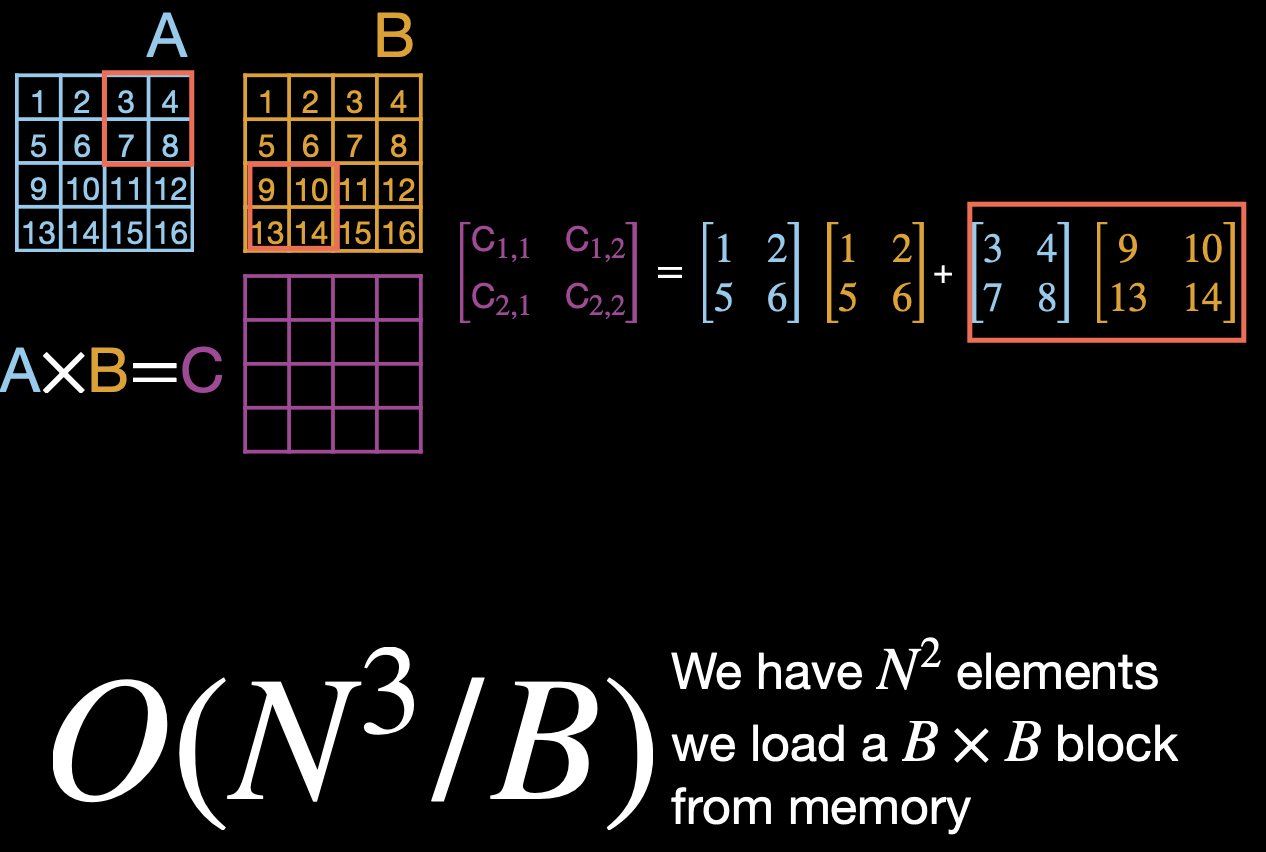
The complexity now decreases to $O(N^3/B)$ since we load $B\times B$ blocks from memory.

So for before, $S$ and $O$ will be computed with tiling, but for $A$ we will need the sum of the individual row.

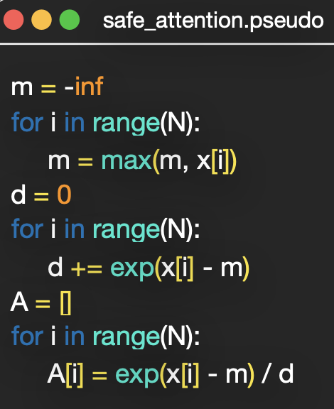
$exp$ is not numerically stable in binary floating point. The fix is stable softmax, which is removing the max of $S$ from the row sequence. You scale the values to the negative, the max will be 0, and by applying the exponential, we scale into a much smaller range than before. He lost me at $m_i$ and $m_N$. It’s about optimizing the second loop of $d$. Finally it comes down to a recursive formulation. Apparently you can also include the computation of $O=AV$ in these loops.

clarifying the stable softmax idea:

Plain softmax needs the whole row before I can normalize:

$$softmax(x{)}_i=\frac{e^{x_i-m}}{{\sum }_j{e}^{x_j-m}}$$

I need max and sum over the entire row of $S$. But tiling only gives me one chunk of the row at a time.

So how do I compute a correct softmax without seeing the whole row at once?

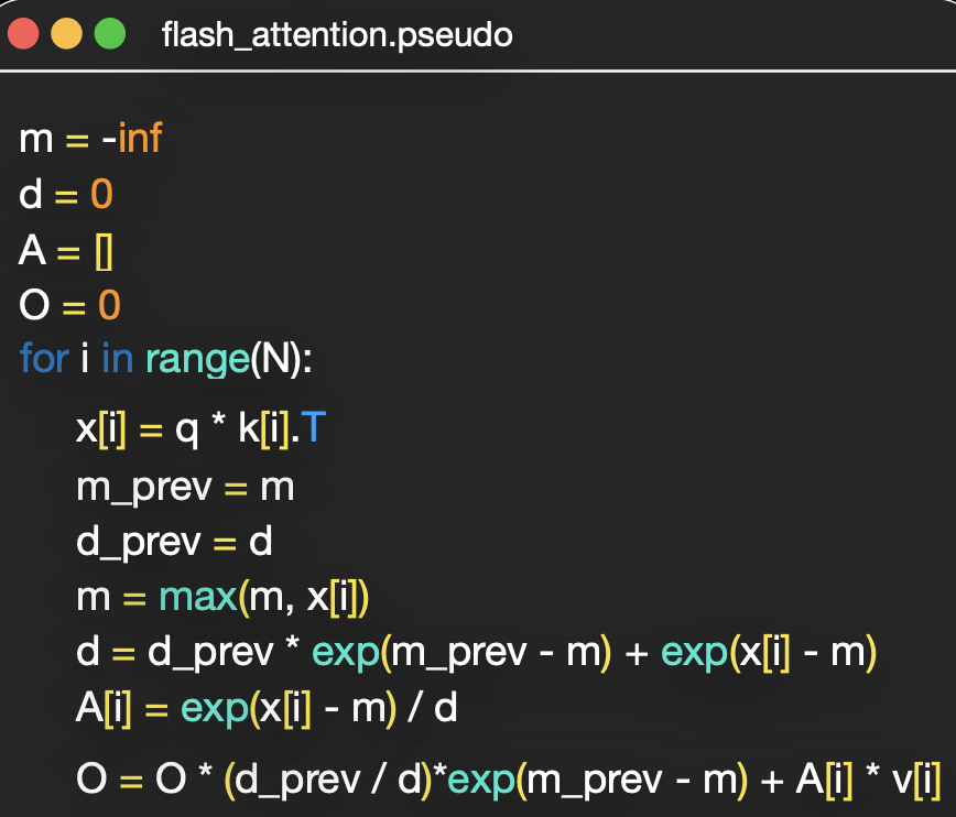
Trick: keep a running max m and running sum l, and correct my previous partial output whenever a new tile reveals a bigger max. Concretely, after processing tiles 1..j, I track:

• $m_j$ = max seen so far
• $d_j$ = sum of $exp(x-m_j)$ so far, correctly rescaled
• $O_j$ = output accumulated so far, correctly rescaled

When tile j+1 arrives with new max candidate, we take it into consideration and update

The mechanism above corresponds to Flash Attention which gets the job done in only one loop $O(n)$.

KV caching is storing the keys and values in the cache memory. Required memory: $2\times K{V}_{dim}\times Precision\times Num.Heads\times Nm.Layers\times Seq.Len$.

• $2\times 128\times 2\text{bytes/head}\times 128\text{heads}\times 61\times 32768=131GB$

This is where experts make the difference. They understand these things when designing neural networks. For the entire formula, the one thing we can control easily is the number of heads, i.e. Multi-Query Attention (MQA) which means use only one head for the keys and the values (validate this).

• With MHA we might need 4MB for KV cache,
• With MQA we need only 31kB (128 $\times$ reduction),
• With GQA we need 500kB.

Can we find a better balance?

yes. Use batches, i.e. Group Query Attention (GQA). Very popular.

Try to understand the Multi-Head Latent Attention (MLA) where you break the process in two (compress and up-project everything).

$$(MLA)d_c<<D\times h\times KV(MHA)$$

See the slide with the comparison between what each technique stores (kB, MB). With MLA it even works better than MHA (so this is the most efficient way of doing it).

MLA is the new norm, not MHA.

It is both faster and better in results. Since 1-2 years.

MLA requires 70kB KV cache per token.

Method	What it does	Cache size
MHA (Multi-Head Attention)	every head has its own K, V	~4MB
MQA (Multi-Query Attention)	all query heads share one K, V head	~31kB (128x smaller)
GQA (Grouped-Query Attention)	query heads share K, V in small groups	~500kB (middle ground)
MLA (Multi-Head Latent Attention)	compress K, V into a small latent vector, up-project when needed	~70kB, but better quality than MHA

---

Softmax?

Currently we know about $o_t={\sum }_{j<t}\frac{exp(q_t{k}_j^{\top })}{exp(q_t{k}_l^{\top })}{v}_j$ which requires storing all past $K,V$ (O(L) memory) because the softmax normalization mixes everything together. We need to escape the $exp$ function i.e. converting to linear attention.

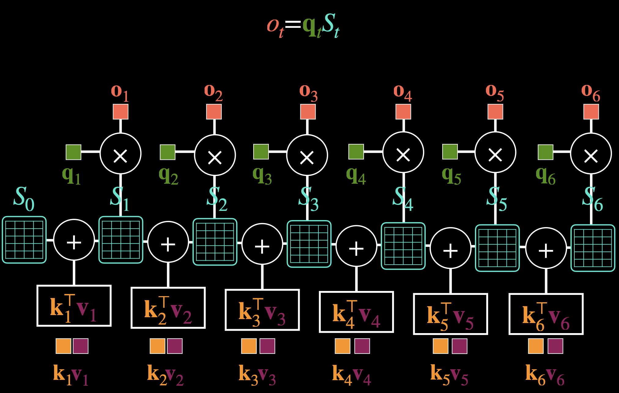
State matrix $S_t={\sum }_{j<t}{k}_j^T{v}_j=S_{t-1}+k_j^T{v}_j$. Again, recursion. Insert the slide he has on the computations. Again, smart. This is Linear Attention which replaces Softmax Attention with plain dot product.

• Softmax Attention:
  • Store KV in memory
  • $O(L)$ memory
• Linear Attention:
  • Store $S_t$ in memory
  • $O(1)$ memory (only update the state)

But linearity includes challenges. There’s no real parallelism possible since each state comes as keys and values come along. There’s also a lot of cost in updating the states (high I/O costs for state updates).

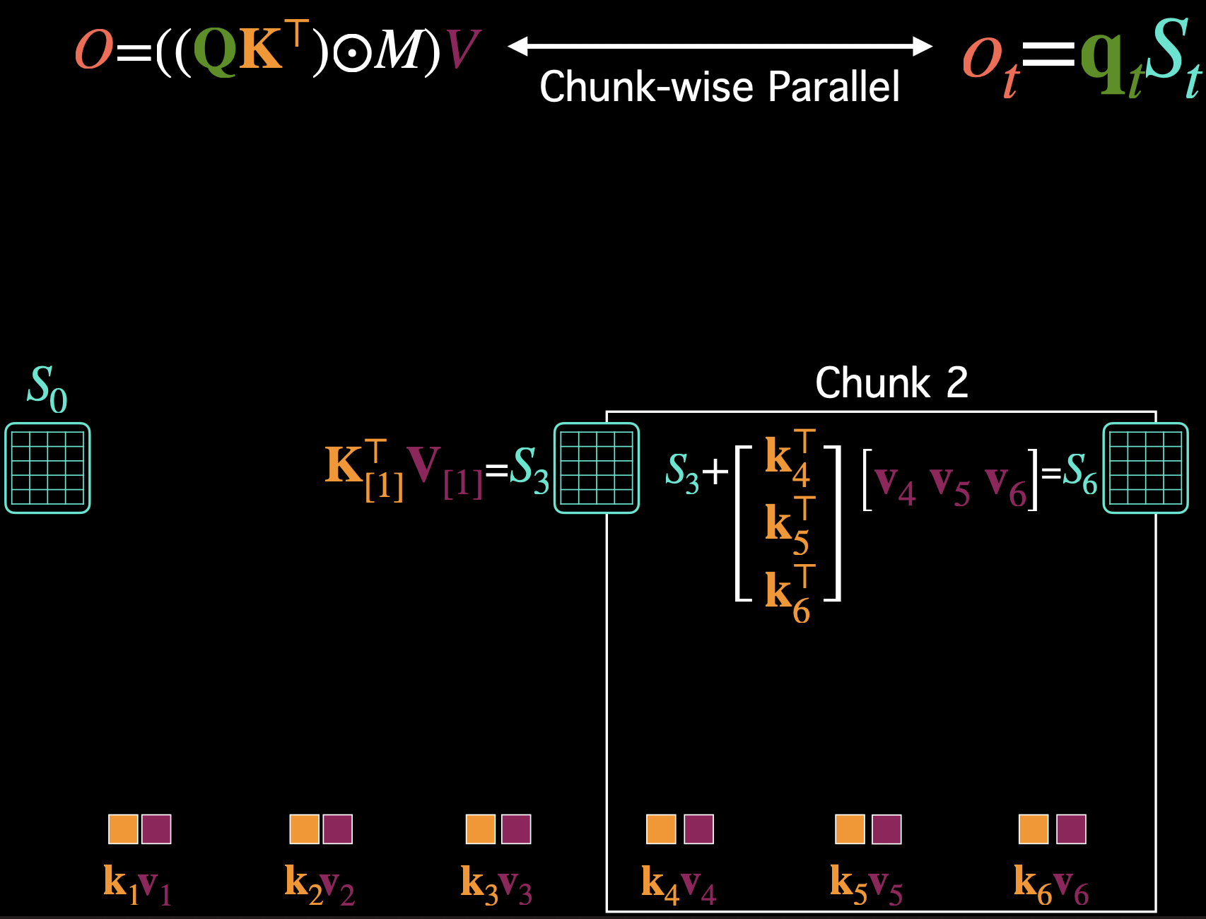
Chunk-wise parallelism

instead of computing every single state, we can just compute individual steps. The first chunk could go from S0 to S3 and compute the instant $k_j^T{v}_j$ in parallel. We can just do a vector multiplication in this case $S_3=K_{0:3}^T\times V_{0:3}$. Hopefully it makes sense. And then we go from 3 to 6 and so on.

Next he talks about moving the key vector close to the value vector through $\hat{v}=kS$ and then compute the loss function with SDG update at t. See delta update rule for linear attention, that’s how he formulates it. So the idea is to train $S$ to be the operator that maps keys to their values. This loss is small when $k_{t}S\approx v_t$, i.e. when my current state $S$, applied to key $k_t$, successfully predicts/reconstructs $v_t$.

$$L_t(S)=-(k_{t}S{)}^{\top }{\mathbf{v}}_t\text{loss at t}$$ $$S_t=S_{t-1}-{\beta }_t\nabla L_t(S_{t-1})\text{SDG update at t}$$ $$S_t=S_{t-1}+{\beta }_t{k}_t^{\top }{\mathbf{v}}_t$$ $$S_t=S_{t-1}+{\beta }_t{k}_t^{\top }({\mathbf{v}}_t-k_t{S}_{t-1})\text{Delta update rule}$$

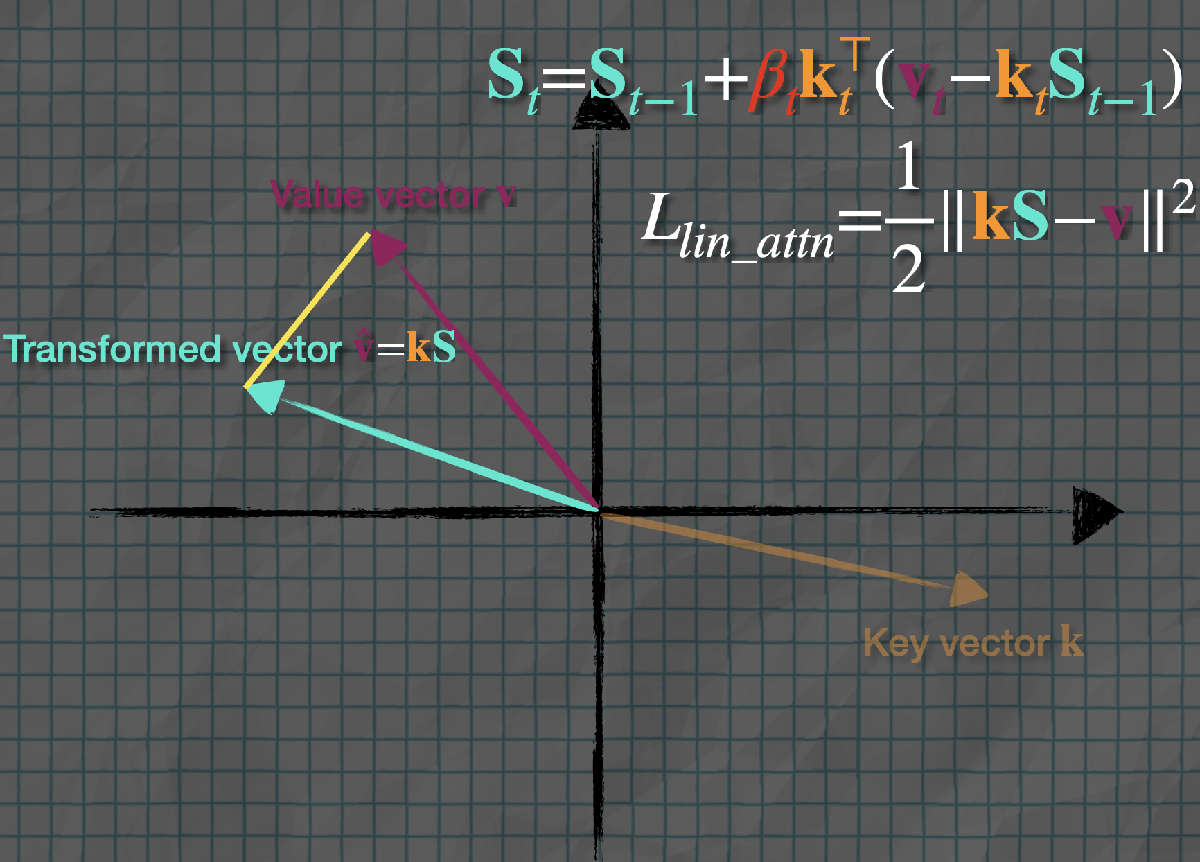
The difference is that istead of just adding $k_t^{\top }{v}_t$ (which can pile up redundant info), it adds the error term $v_t-k_t{S}_{t-1}$ — i.e. only update $S$ by however much it’s currently wrong about predicting $v_t$.

---

RMSNorm

Attention captures token dependencies. However, it’s not enough for retrieving factual information.

look again over this and understand the concept which constrains to a unit sphere. Well, it’s better explained now in Transformers in depth and time. It’s the idea of representing tokens as particles on a sphere. The prior claim (“attention captures dependencies but isn’t enough for factual retrieval”) is gesturing the idea that MoE/expert layers are what store factual/parametric knowledge, while attention handles relational/contextual mixing.

Routing / Mixture of Experts

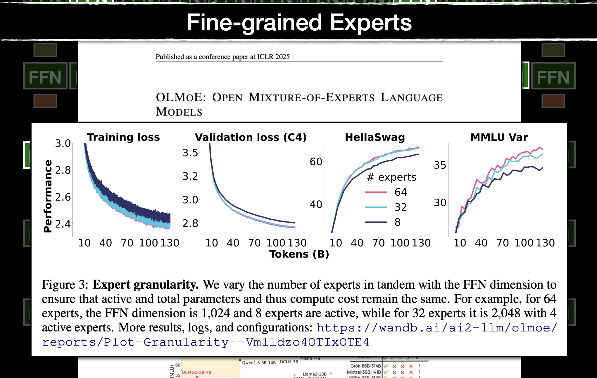
See OLMoE to understand the experts explanation he gave. From 2024 (GPT 3.5 nano) onwards, everything is a mixture of experts.

Idea of Mixture of Experts (MOE): learn E separate MLPs per block; route each token to $A<E$ active experts. Increases total params by $E$, compute by only $A$. Almost every frontier LLM today (GPT-4o, Claude, Gemini) is believed to be MoE with >1T params.

instead of every token passing through the same dense FFN, route each token to a small subset of “expert” FFNs.

$$\text{Expert capacity}=\frac{\text{Total tokens in a batch}}{\text{Number of experts}}\times \text{Capacity factor}$$

Intuition: most parameters are “dormant” for any given token. Each token only pays for the handful of experts relevant to it, so total capacity scales without paying FLOPs for every parameter

token overlflow: tokens are dropped. Each expert can only handle a fixed number of tokens per batch (its “capacity”). If more tokens get routed to one expert than it has capacity for, the overflow tokens are simply dropped (skip that expert, e.g., passed through via a residual/skip path)