Self-Supervision Objectives for FoMo Pre-training

This lecture covers 4 families of pretext tasks for self-supervised pre-training.

The big picture is that, instead of labels, we invent a pretext task that forces the network to learn useful representations from raw data alone, then transform those features to real downstream tasks.

invariance-based methods = apply a bunch of augmentations to the original image, and make sure the embeddings generated from those images are very similar (invariant to augmentations)

Pretext task 1: Vision-language score — CLIP $\to$ SigLIP $\to$ GLIP

• CLIP: encode image and text in the same space. The similarity between two normalized vectors simply comes down to their cosine similarity, which is what CLIP maximizes. The temperature $\tau$ is a hyperparameter which helps with numerical stability (controls how peaked the softmax/exponential output is).
  • Dividing by a small $\tau \sim 0.07$, we get a sharper and more confident distribution, as small similarity differences get amplified into big probability differences
  • Dividing by a big $\tau$, we get a softer distribution; where differences get washed out.
  • So basically, scaled so gradient are informative rather than mushy. In DINO, the teacher temperature is smaller so its output is sharper/more confident than the student’s.

$$L_{\text{CLIP}}=-\frac{1}{N}(\underset{\text{Image-to-Text Loss}}{\underbrace{\sum _i\ln \frac{e^{v_i\cdot w_i/\tau }}{{\sum }_j{e}^{v_i\cdot w_j/\tau }}}}+\underset{\text{Text-to-Image Loss}}{\underbrace{\sum _j\ln \frac{e^{v_j\cdot w_j/\tau }}{{\sum }_i{e}^{v_i\cdot w_j/\tau }}}})$$

• SigLIP: an improved version of CLIP which introduces sigmoid-based contrastive loss instead of the traditional softmax-based contrastive loss. This training loss eliminates the need for a global view of all pairwise similarities between images and texts within a batch. It transforms the problem into $N^2$ independent binary classifications. Since we don’t need to gather everything onto one device before computing the loss ⇒ much easier to scale to huge batch sizes across many GPUs .Consequently, it enables more efficient scaling to larger batch sizes while also delivering superior performance with smaller batch sizes.
  • also introduces a learnable bias ($b$) to offset the huge negative-to-positive ratio. Because out of $N^2$ pairs per batch, only $N$ are positive. That’s what $b$ is for — a learned bias that shifts the decision threshold so the sigmoid isn’t just trivially predicting negative for everything to minimize loss.
  • $z_{ij}$ is the ground-truth label.
  • TL;DR: Cheaper, scales better.

$$L_{\text{SigLIP}}=-\frac{1}{N}\sum _i\sum _j\ln \frac{1}{1+e^{z_{ij}(v_i{w}_j/\tau +b)}},z_{ij}=\{\begin{array}{ll}1& \text{if }{v}_i\text{ and }{w}_j\text{ are paired}\\ -1& \text{if }{v}_i\text{ and }{w}_j\text{ are not paired}\end{array}$$

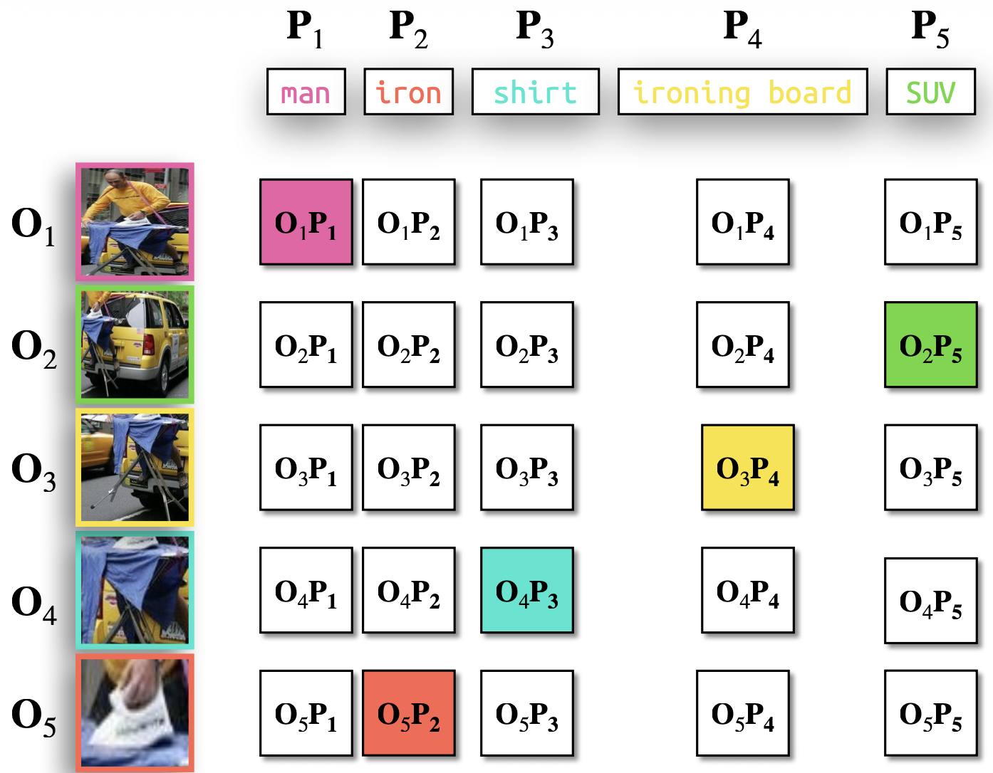
• GLIP (Grounded Language-Image Pre-training): unifies object detection and text-image grounding. It extends alignment from whole-image/whole-caption to region $\leftarrow \to$ phrase grounding
  • compute a similarity matrix between detected object regions (O) and text phrases (P), add a localization loss on top of the classification loss.

$$L_{\text{GLIP}}=\underset{\text{Binary-Sigmoid Multi-Class Classification}}{\underbrace{L_{\text{cls}}}}+\underset{\text{Centerness Loss \& Edge Distances}}{\underbrace{L_{\text{loc}}}}$$

Phrase Grounding

the process of mapping specific words or textual phrases to their representations within an image or video

---

Pretext task 2: Negative samples (Contrastive) — SimCLR $\to$ MoCo

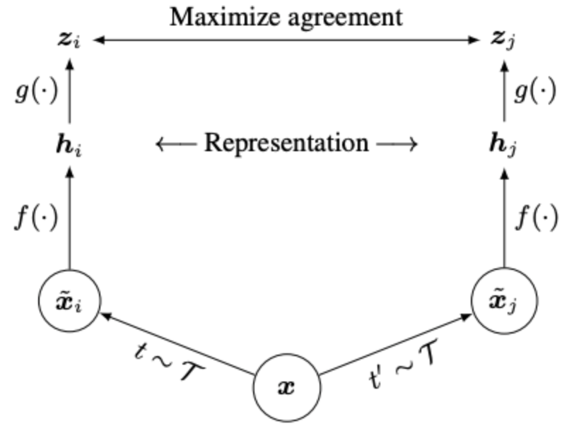
• SimCLR (Simple framework for Contrastive Learning of visual Representations): Two separate data augmentation operators ($t\sim \tau$ and $t^{\prime }\sim \tau$) are applied to each data example to obtain two correlated views. A base encoder network $f(\cdot )$ and a projection head $g(\cdot )$ are trained to maximize agreement using a contrastive loss. After training we throw away $g$ and use encoder $f$ and representation $h$ for downstream tasks.
  • The pipeline: $x\stackrel{t\sim \mathcal{T}}{\to }{\tilde{x}}_i\stackrel{f(\cdot )}{\to }{h}_i\stackrel{g(\cdot )}{\to }{z}_i$
    • $\mathcal{T}$ is the augmentation distribution (random crop + color distortion + Gaussian blur + invert + flip .. etc. first three I think are crucial)
    • $z$ is where the contrastive loss is applied. Representation $z$ is trained to be invariant under augmentation — that collapses useful signal (e.g. color, orientation). $h$ sits one MLP away, so it keeps information that $z$ had to throw out. Linear eval on $h$ beats linear eval on $z$ consistently; SimCLR ablation table shows non-linear projection head $\sim 7$ points better than no head.
  • Minibatch algorithm: For a minibatch of $N$ images:
    • 1. Draw $t,t^{\prime }\sim \mathcal{T}$, apply both to every image ⇒ $2N$ augmented views
    • 2. Encode with shared encoder + projection $\to$ $z\in {\mathbb{R}}^{2N\times D}$.
    • 3. Build affinity matrix $s_{i,j}=z_i^T{z}_j/(||z_i||||z_j||)$ — cosine similarity, shape $2N\times 2N$. $B=N$.
    • 4. For each row $i$, the positive is at position $2k$ or $2k+1$ (partner view of the same source image); all other $2N-2$ entries are negative.
    • 5. InfoNCE per row: $l(i,j)=-\log \frac{\exp (s_{i,j}/\tau )}{{\sum }_{k\ne i}\exp (s_{i,k}/\tau )}=-\log \frac{e^{\text{sim}({\mathbf{z}}_i,{\mathbf{z}}_j)/\tau }}{{\sum }_{k\in 2B}{e}^{\text{sim}({\mathbf{z}}_i,{\mathbf{z}}_k)/\tau }}$
    • Total loss averages $l(2k,2k+1)+l(2k+1,2k)$ over all $N$ source images. Quality scales with number of negatives, which scales with batch size $B\to O(B^2)$ compute, which makes it infeasible at scale. That’s where MoCo comes in.

• MoCo (Momentum Contrast for Unsupervised Visual Representation Learning): In SimCLR, to get lots of negatives you need a huge batch ($8k\to$ TPU pods). MoCo sidesteps this by decoupling negative count from batch size(key difference to SimCLR) by keeping a momentum-updated key encoder (EMA of the query encoder, no gradients), and a queue of past keys as negative dictionary ⇒ $O(B\times K)$ instead of $O(B^2)$. Only the query encoder gets backprop; the key encoder is updated via ${\theta }_k\leftarrow m{\theta }_k+(1-m){\theta }_q$
  • Queue mechanics: Maintain a dictionary $\{k_0,k_1,k_2,\dots \}$ of size $K$ (e.g. 65536). Each iteration:
    • Encode curent minibatch’s key view with the momentum encoder $\to$ enqueue.
    • Dequeue the oldest minibatch’s keys
    • The queue acts as a large, slowly-evolving dictionary of negatives. No gradients flow into it.
  • Momentum update:
    • Let ${\theta }_q$ be the query-encoder params, ${\theta }_k$ key-encoder params: ${\theta }_k\leftarrow m{\theta }_k+(1-m){\theta }_q,m=0.999{\theta }_k$ changes slowly — essential for queue consistency, because the keys in the queue were encoded by slightly older ${\theta }_k$ and a fast-moving key encoder would make them stale.
  • MoCo v2 — hybrid with SimCLR: pulls SimCLR’s two best ideas into MoCo’s framework
    • Non-linear MLP projection head (SimCLR’s $g(\cdot )$).
    • Strong data augmentation (+Gaussian blur).
  • MoCo v3: adapts MoCo to ViT backbones, studies training stability.

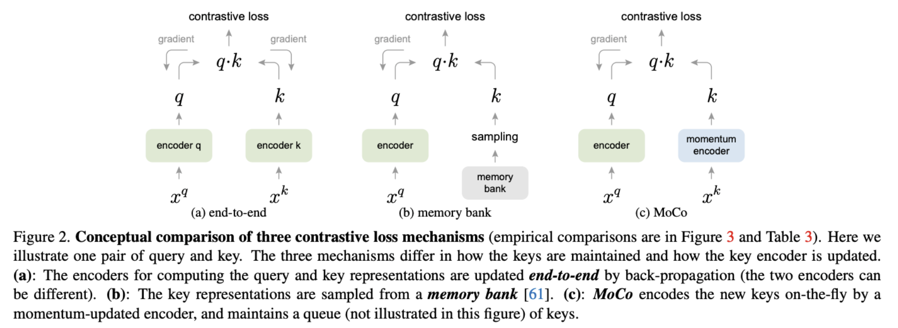
MoCo vs SimCLR

	SimCLR	MoCo
Source of negatives	other samples in current minibatch	FIFO queue of keys from many past minibatches
Key encoder	shared with query encoder	momentum encoder (no gradients)
Gradient flows	through both views	only through the query
Practical	needs batch 8192 on TPU	works at batch 256 on 8 V100s

MoCo Pseudocode

for x in loader:
    x_q, x_k = aug(x), aug(x)
    q = f_q.forward(x_q)          # N x C
    k = f_k.forward(x_k).detach() # N x C, no grad through key
    
    l_pos = bmm(q.view(N,1,C), k.view(N,C,1))   # N x 1
    l_neg = mm(q.view(N,C), queue.view(C,K))    # N x K
    logits = cat([l_pos, l_neg], dim=1)          # N x (1+K)
    
    labels = zeros(N)                             # positive is at index 0
    loss = CrossEntropyLoss(logits / tau, labels) # InfoNCE
    
    loss.backward()
    update(f_q.params)
    
    f_k.params = m * f_k.params + (1 - m) * f_q.params  # momentum update
    enqueue(queue, k); dequeue(queue)
 

---

Pretext task 3: Self distilation — DINO

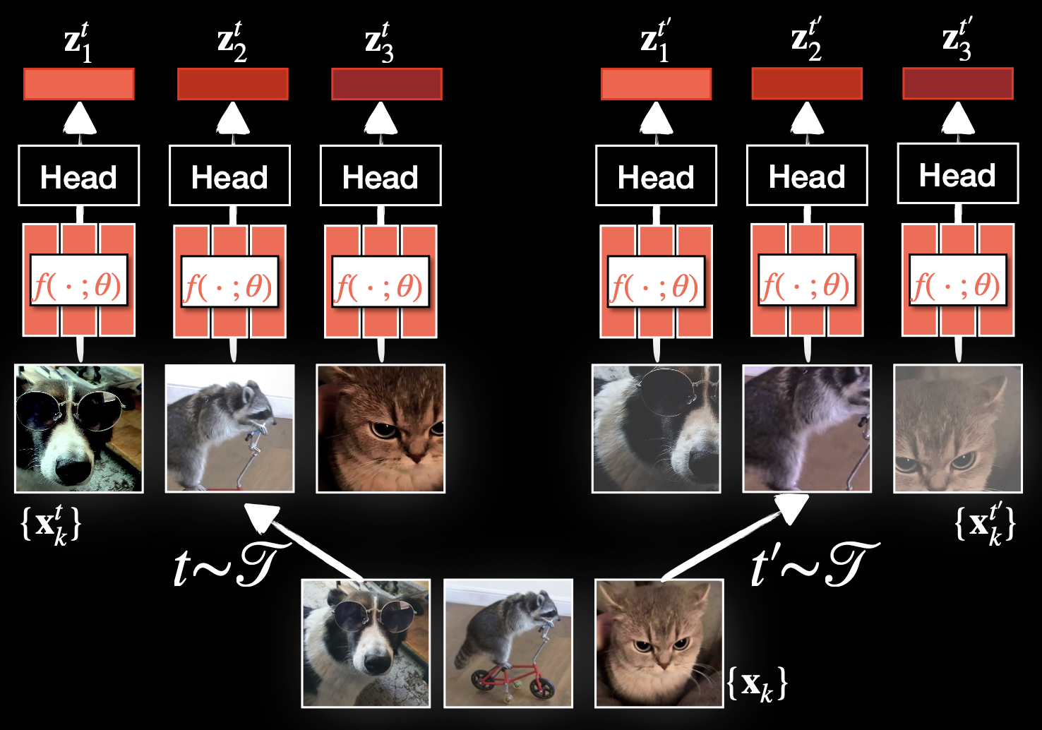
• DINO: no negatives at all. Student and teacher share architecture. teacher = EMA of the student. Both produce a softmax distribution over $K$ prototype dimensions on different crops of the same image; student is trained to match the teacher’s distribution (cross-entropy), gradient only flows through the student.
• here just complete with equations explanations and size of variables for pseudocode.

---

Pretext task 4: Low-level targets — MAE, BEiT, I-JEPA

TL;DR: Split image into patches, mask most of them, encode the visible ones, try to recover what’s missing.

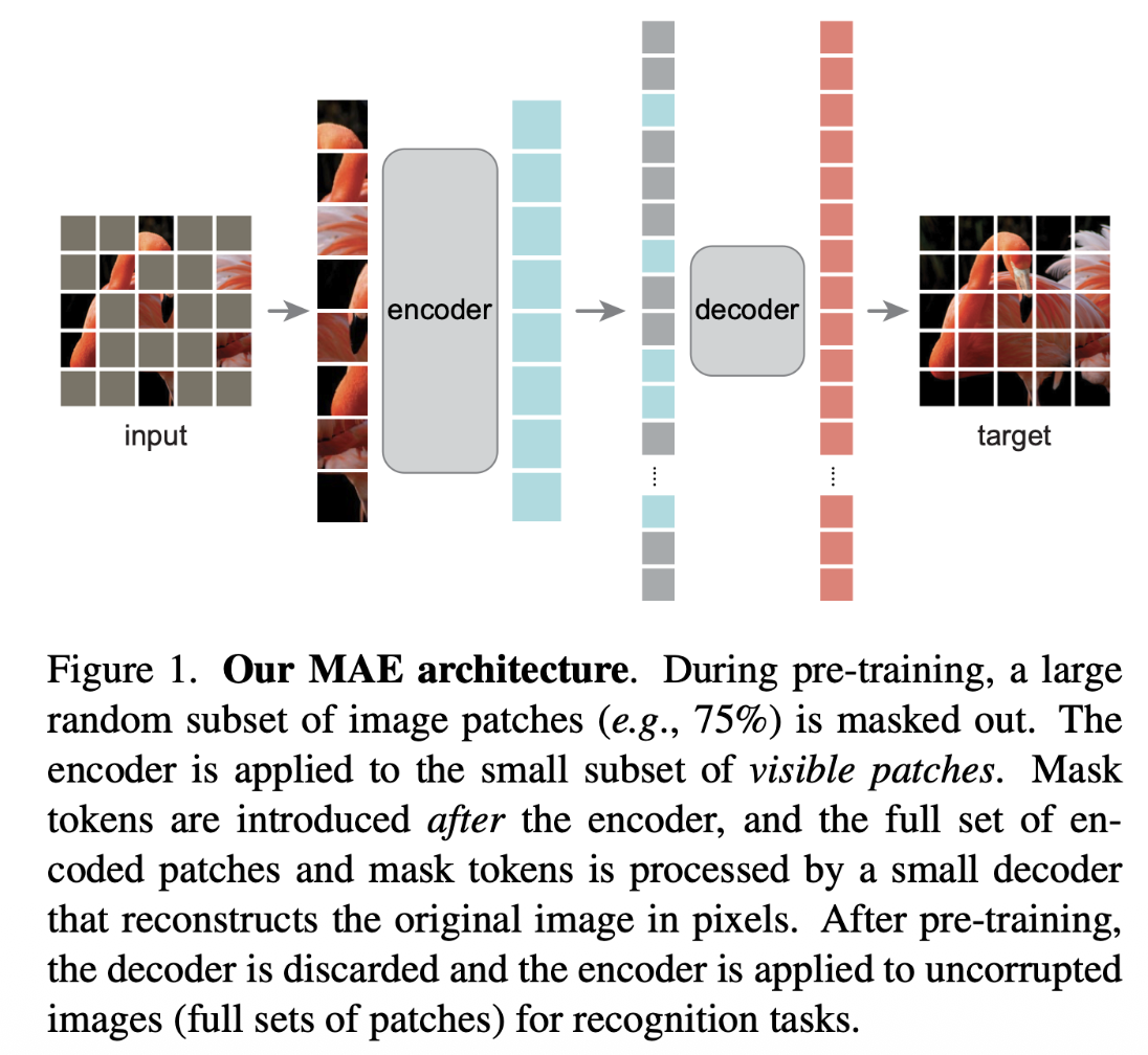
• MAE (Masked Autoencoders): reconstruct raw pixels of masked patches, L2 loss $L_{\text{MAE}}=||{\mathbf{x}}_p-\widehat{{\mathbf{x}}_p}|{|}_2$.
  • asymmetric encoder-decoder architecture.
    • encoder operates only on the visible subset of patches
    • lightweight decoder that reconstructs the original image from the latent representation and mask tokens. Decoder is much lighter than encoder. After pre-training, throw the decoder away.
  • masking a high proportion of the input image (e.g. 75%) yields a meaningful self-supervisory task.
  • i.e. split image $\mathbf{x}$ into patches ${\mathbf{x}}_p$ $\to$ select a random set of patches ${\mathbf{x}}_p^{\prime }\sim {\mathbf{x}}_p$ $\to$ Linear Project: $pro{j}_i={\mathbf{x}}_i^{\prime }\times w+b$
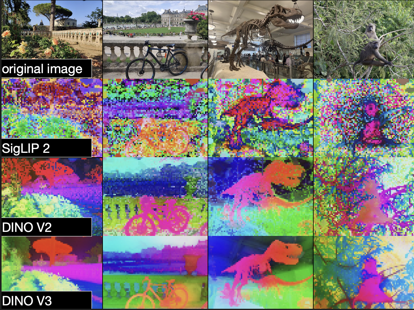
  • results are quite blurry, because it sort of learns the mean.

How can masked autoencoding work so well without diffusion? -- Steven

MAEs don’t need to generate an image pixel-by-pixel from pure noise (like diffusion).

They start with a partially observed image: a small set of visible patches already gives a huge amount of structure (object shapes, colors, layout).

The model’s job is to fill in the missing patches so the whole image is coherent — this is a much lower-entropy task than unconditional generation.

• BEiT (BERT Pre-Training of Image Transformers): reconstruct a discretized visual token (codebook index) instead of raw pixels.
  • $L_{\text{BEiT}}=||pro{j}_p-{\widehat{proj}}_p|{|}_2$
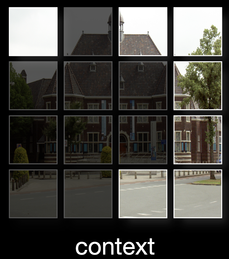
• I-JEPA (Image-based Joint-Embedding Predictive Architecture): don’t reconstruct pixels/tokens at all — predict the embedding of the masked patches, produced by an EMA target encoder, using a separate predictor network.
  • pixel-level reconstruction wastes capacity on irrelevant low-level detail; predicting in latent space is more efficient. This is the bridge between “low-level targets” and “self-distillation” (it borrows the EMA-teacher trick from DINO but applies it to masked prediction). JEPA never tries to reconstruct pixels, nor to model the full joint distribution of natural images. It only tries to predict representations of masked parts of the same image.
  • context encoder $f(\cdot ,{\theta }_c)$ encodes $z_c$ context latents
  • EMA update: ${\theta }_t\leftarrow m{\theta }_t+(1-m){\theta }_c$
  • ”we leverage an asymmetric architecture between the x- and y-encoders to avoid representation collapse.”

$$L_{\text{MSE}}=\frac{1}{|\mathcal{M}|}\sum _{i\in \mathcal{M}}||z_{p_i}-sg(z_{t_i})|{|}_2^2$$

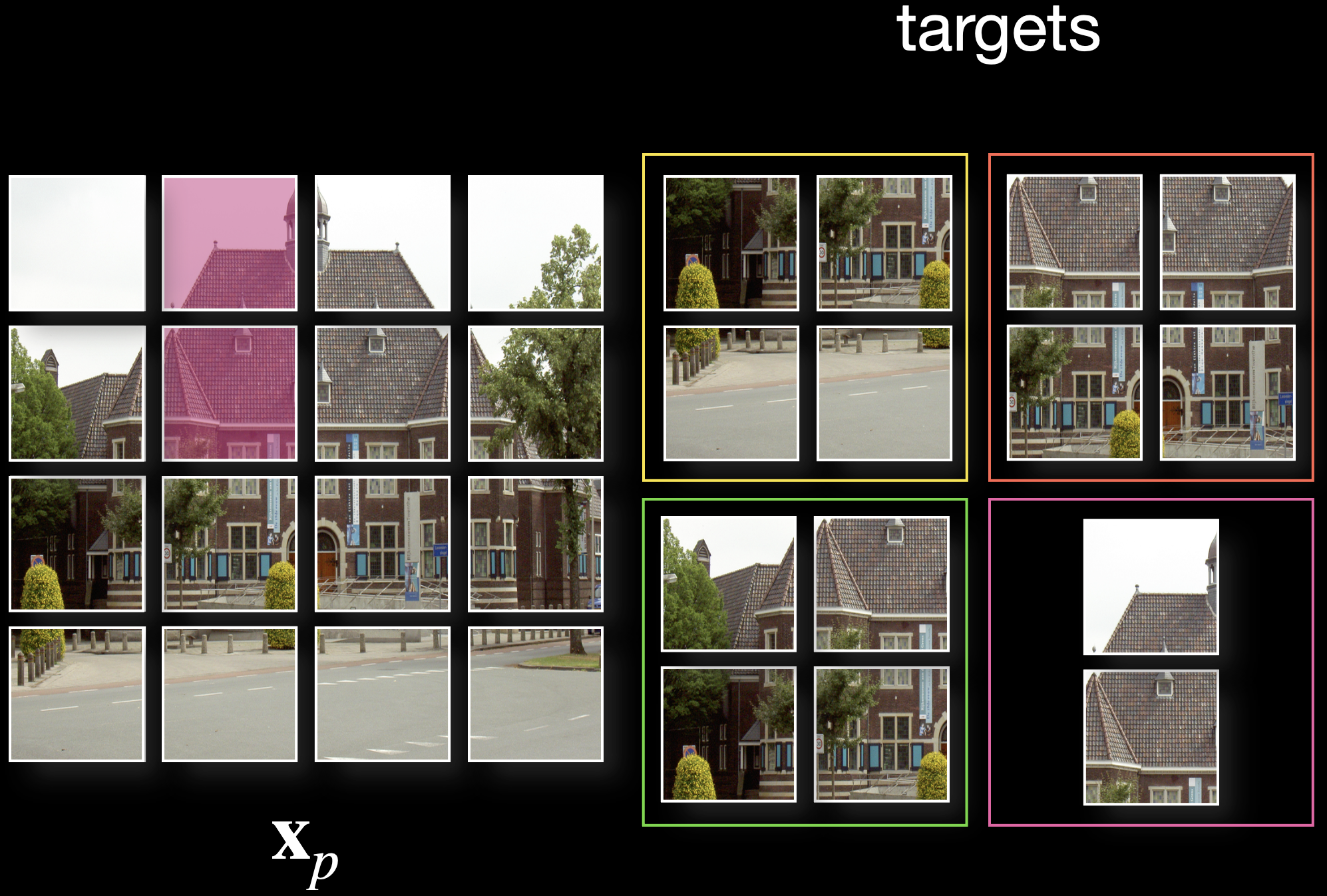
• $z_{p_i}$ — predicted latents for target $i$
• $z_{t_i}$ — targets $i$. $sg()$ because targets should be fixed, so do not compute gradients.
• ${\sum }_{i\in \mathcal{M}}$ — sum over all targets and predictions, $\mathcal{M}$ is target blocks.

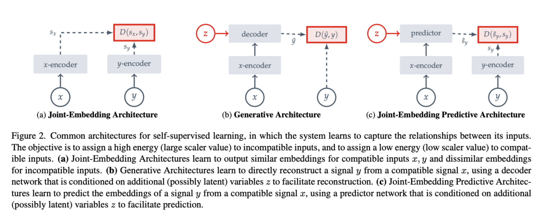
Each architecture

Joint-embedding architecture

• A big limitation is representation collapse.
• Collapse-prevention based on architectural constraints leverage specific network design choices to avoid collapse, for example, by stopping the gradient flow in one of the joint-embedding branches, using a momentum encoder in one of the joint-embedding branches, or using an asymmetric prediction head

Generative architecture

$x$ is a copy of $y$, but with some of the patches masked. $z$ corresponds to a set of mask and position tokens to specify to the decoder which image to reconstruct. Representation learning is not an issue

JEPA

In contrast to Joint-embedding architectures, JEPAs do not seek representations invariant to a set of hand-crafted data augmentations, but instead seek representations that are predictive of each other when conditioned on additional information $z$.

• still suffer from representation collapse