Autoencoders

Lecture 2 from my GenAI Models and Robotic Applications course.

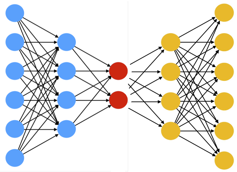
Encoder

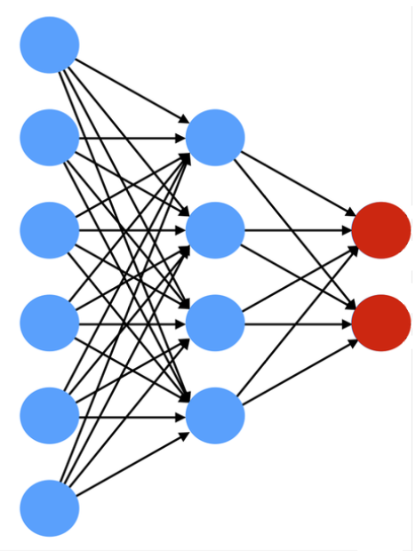
• From high dimensions to low dimensions
• A function that encodes an input sample into a lower-dimensional code
• Fully-connected
• Convolutional
• Sparse

Decoder

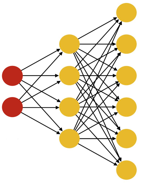
• From low dimensional space to higher dimensional space
• A function that encodes an input sample into a higher-dimensional code
• Fully-connected
• Convolutional
• Sparse
• Convolutional decoders perform transposed convolutions or upsampling and convolutions to reverse the downsampling of the decoder.

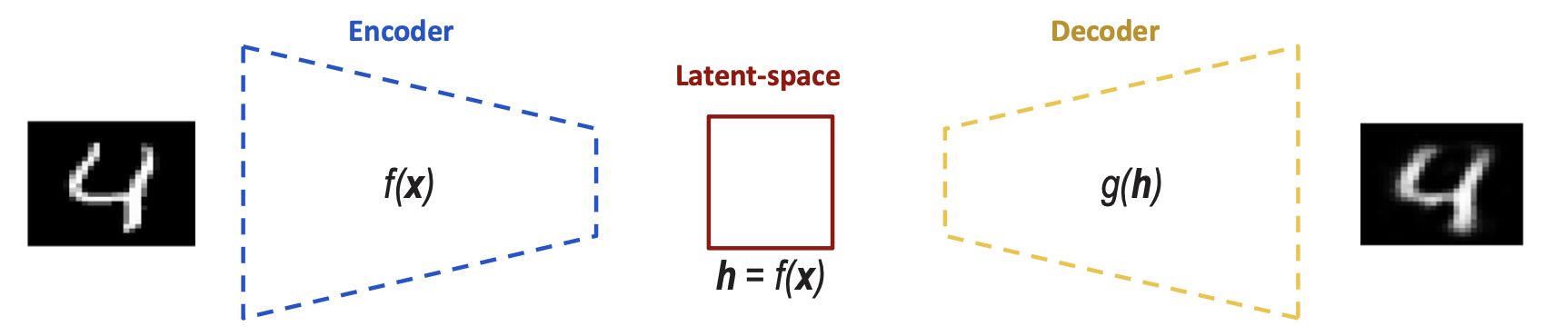
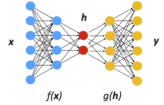
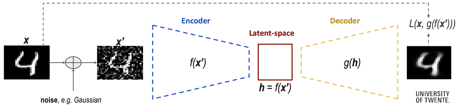
Autoencoder (AE)

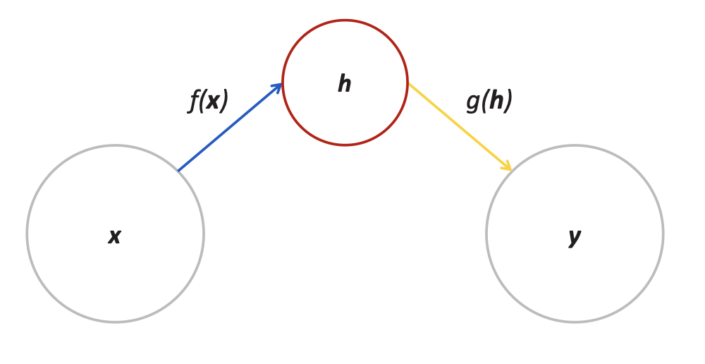
• f(x) is the encoding function
• g(h) is the decoding function
• h is the latent space. Here we can use it to learn more about the information (extraction and probably compression or even manipulating this data e.g. features for classification)
• the learning process is described as minimizing a loss function $L(x,g(f(h)))$

• A neural network with the task of copying the input to the output (difference between x and g(f(h)) is 0)
• Trained to minimize the dissimilarity between the original input sample(s) and the reconstructed output
• Convolutional decoders perform transposed convolutions or upsampling and convolutions to reverse the downsampling of the decoder.

it’s a way to learn features in an unsupervised way.

Visualizing the latent space of an AE

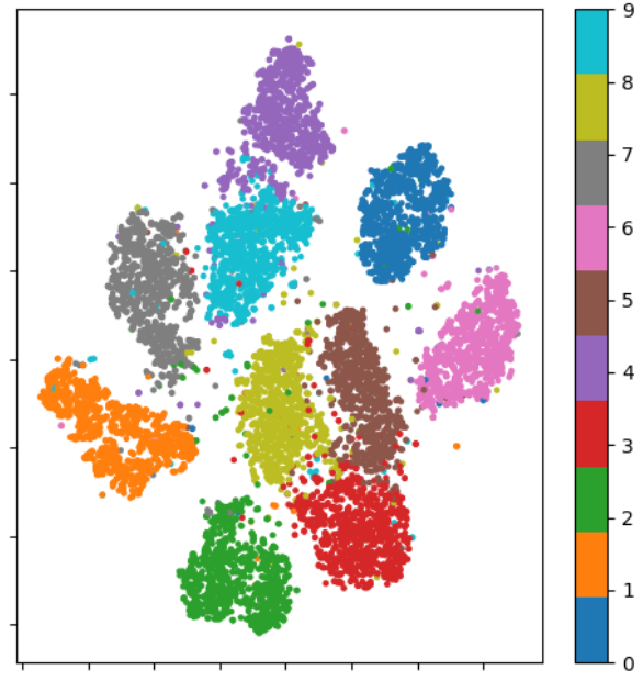
• An AE maps the input samples to points into the latent space, building large mutually independent clusters (no relations between the 'neighbor' clusters)
• The mapping is optimized to reconstruct the input samples only.

Problems

• When the hidden layer h has the same dimension as input x, the network can cheat by just copying the input. If the encoder/decoder are too large, they memorize training samples instead of learning meaningful patterns.

Solution: Undercomplete Autoencoders

Undercomplete AutoEncoders

• The hidden layer h is deliberately smaller than the input x (|h| << |x|). This forces the network to compress the input, learning only the most important features for the training distribution.
• Main Application: Dimensionality Reduction

• Benefits: Prevents trivial identity learning, creates useful compressed representations,
• Limitation: The learned features are optimized for the training distribution and may not generalize to diverse inputs,
• The encoder and decoder must have limited capacity. If they're too powerful (even with a 1D bottleneck), the decoder can still memorize by mapping each training example to a unique integer index, defeating the purpose of compression.

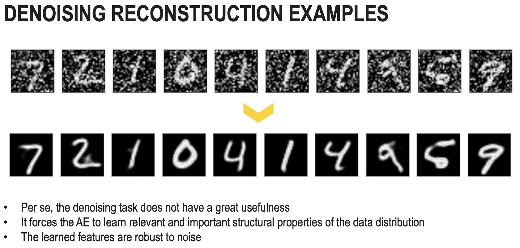
Denoising AutoEncoders (DAE)

• Trained to remove noise from the image. DAEs are trained to take a (partially) corrupted input and recover the original undistorted input.
• We take the input(x), we corrupt it with noise(x’) and it becomes the input for the encoder. Train by minimizing the MSE loss between original and reconstructed samples.
• DAE learns features that catch important structures in the input distribution of the training data.

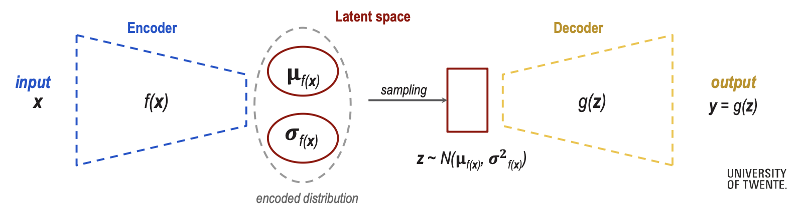
Variational AutoEncoders (VAE)

• Based on variational inference theory
• Enforces the learning of a regularized latent space (with a probabilistic twist)
• Does not encode inputs as points, but as a distribution over the latent space.
  • The latent code is sampled from the learned distribution
  • The decoder reconstructs the sampled distribution points

The mean and standard deviation are now in high dimensional space (variance is the covariance matrix and the mean is also a matrix).

• E[$log{p}_g(x\mid z)$] is the entropy loss.
• $D_{KL}$ is a measure of difference between distributions.
• Aim is to reconstruct the input accurately and enforcing a known distribution to the latent space

$${\mathcal{L}}_{ELBO}(x,f,g)=E[\log p_g(x|z)]-D_{KL}(q_f(z|x)||p(z))$$

Sampling does not flow back (Backpropagation through randomness is not possible). That’s why we have to do a reparametrization trick: Separate the randomness from the learnable (and differentiable) parameters $z=\mu +\sigma \cdot ϵ$, where $ϵ\approx N(0,1)$, instead of $z\approx N({\mu }_{f(x)},{\sigma }_{f(x)}^2)$

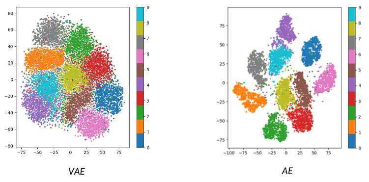
VAE vs AE: latent space

• In the AE latent space, the clusters are not correlated in any way. It’s just a visualization.
• In the VAE latent space, the clusters are correlated through the prior. The KL divergence term pushes all encodings toward $N(0,1)$, which:
  • centers all clusters around the origin
  • Keeps variance controlled
  • Forces the network to use the latent space efficiently
  • Creates semantic relationships — similar digits tend to be closer because they share similar distributions that get pulled toward the same region of the prior. For example, digits 4 and 9 will always sit close to each other when semantic relationships matters.

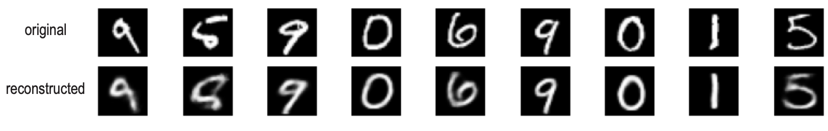
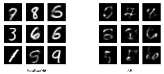
Generation with VAE

• The latent space is encoded as a (Gaussian) distribution.
• Sampling a latent variable ($z$ from $N(\mu ,\sigma )$) and let the decoder generate (reconstruct) an image. VAE produces recognizable digits while AE generates blurry/unclear outputs when sampling randomly.

Latent Space Arithmetic

• Interpolation: Encode two samples (e.g. digit ‘2’ and ‘4’), compute $z_1$ and $z_2$, then interpolate: $z=z_1+\alpha \cdot △$ where $△=z_2-z_1$ and $\alpha \in [0,1]$.
• This results in smooth morphing between digits (2 $\to$ 4) for VAE. In the AE case, we have abrupt jumps with artifacts — the irregular latent space means intermediate points don’t decode meaningfully.

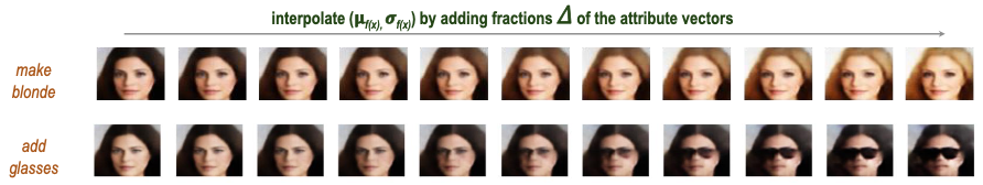
Attribute Manipulation

1. Compute mean latent vectors for each attribute cluster
2. Calculate attribute direction vectors in latent space
3. Add/subtract these vectors to/from an encoded image

Some examples include prompts like “make blonde” or “add glasses” which add or substract the respective vector.

Generative Adversarial Networks (GANS)

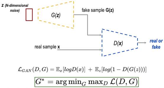
• GANs are generative models based on game theory,
• A generator network G generates fake samples,
• A discriminator network D discriminates between real samples and fake generated samples.

Adversarial Training

$${\mathcal{L}}_{GAN}(D,G)={\mathbb{E}}_x[\log D(x)]+{\mathbb{E}}_z[\log (1-D(G(z)))]$$ $$G^{\ast }=\arg \underset{G}{\min }\underset{D}{\max }\mathcal{L}(D,G)$$

• The two networks compete in a $minimax$ game:
• G minimizes: Makes $D(G(z))\to 1$, fooling the discriminator
• D maximizes: Correctly identifying real ($\log D(x)\to 0$) and fake ($\log (1-D(G(z)))\to 0$)

Conditional GANS (cGANS)

Conditional GANs

• Learning a generator G to reconstruct meaningful samples only from noise z can cause mode collapse(G generates few samples only, D is in a local minimum). Mode collapse means that the training of the network is stuck.
• The solution implies conditioning: Both G and D receive an additional input c (condition) such as a class label, text description, or another image. This guides generation toward specific outputs.

The loss function stays the same but we take c into consideration.

• Generator: $G(z,c)$ — takes noise $z$ and condition $c$
• Discriminator: $D(x,c)$ — evaluates if $x$ is real given condition $c$.

${\mathcal{L}}_{cGAN}(D,G)={\mathbb{E}}_{c,x}[\log D(c,x)]+{\mathbb{E}}_{c,z}[\log (1-D(c,G(z)))]$

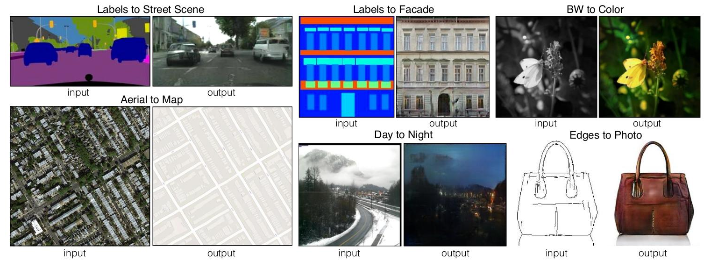
One condition for cGANs in computer vision: ALLIGNMENT (or PAIRED) (the objects are always in the same place). cGANs excel at paired image translation tasks.

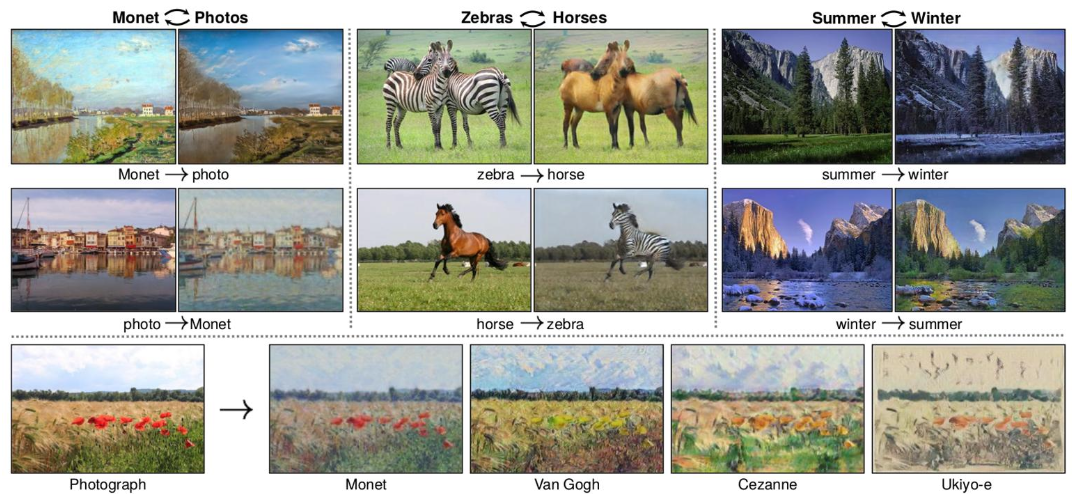
Cycle GANS

• Cycle GANs perform unpaired image-to-image translation: given two unpaired image sets (domains) X and Y, learn a mapping function between the two domains that transforms images from X into images from Y (and vice versa).
• Based on the concept of cycle consistency.
• Paired training samples are difficult to obtain (and scarce).