Object Detection and Tracking

Object Detection

Object detection is:

1. Classification
2. Localization (bbox)
3. Confidence score

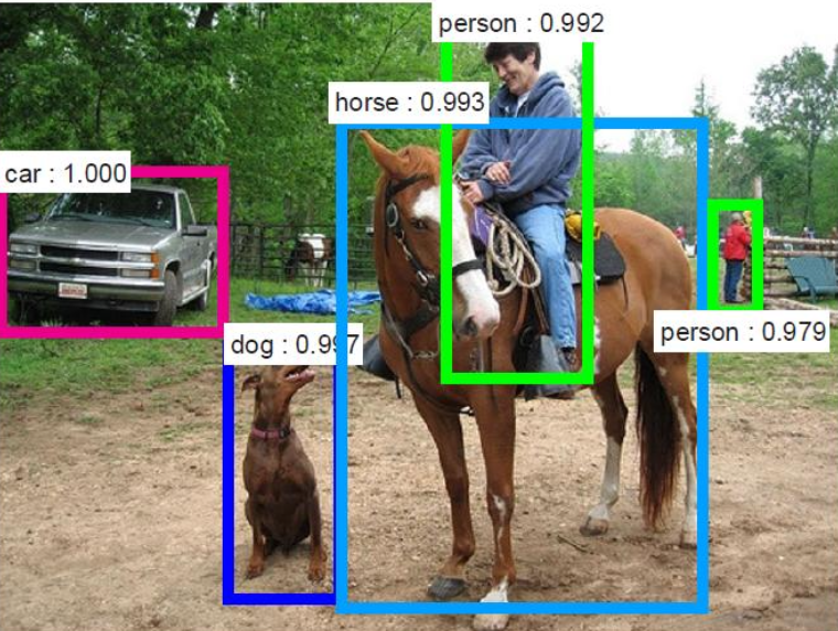
Challenges include: illumination, occlusions, intra-class appearance, viewpoint, etc.

Traditional methods include:

• Sliding window + classifier
• Feature-based methods with handcrafted features

Evaluation metrics include: precision, recall, F score, IoU, AP (Average Precision)

What if we have duplicated bboxes?

NMS removes the low probability predictions (you see which bboxes overlap, and then select the one with the highest score). The IoU should exceed a set threshold.

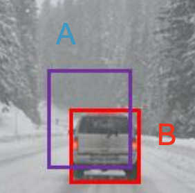
Here, for example, B should get selected as I believe it would yield a better score.

Object Detection Network Architectures

Two Stage Detectors

Faster R-CNN

It’s a two-step classification.

• $1^{st}$ stage would be having a image and applying convolutional layers on that ⇒ feature maps.
• $2^{nd}$ step is a Region Proposal Network (we focus on regions with objects, not empty spaces) ⇒ proposals. Based on the proposals, we crop out the background and then train our classifier to classify the object.

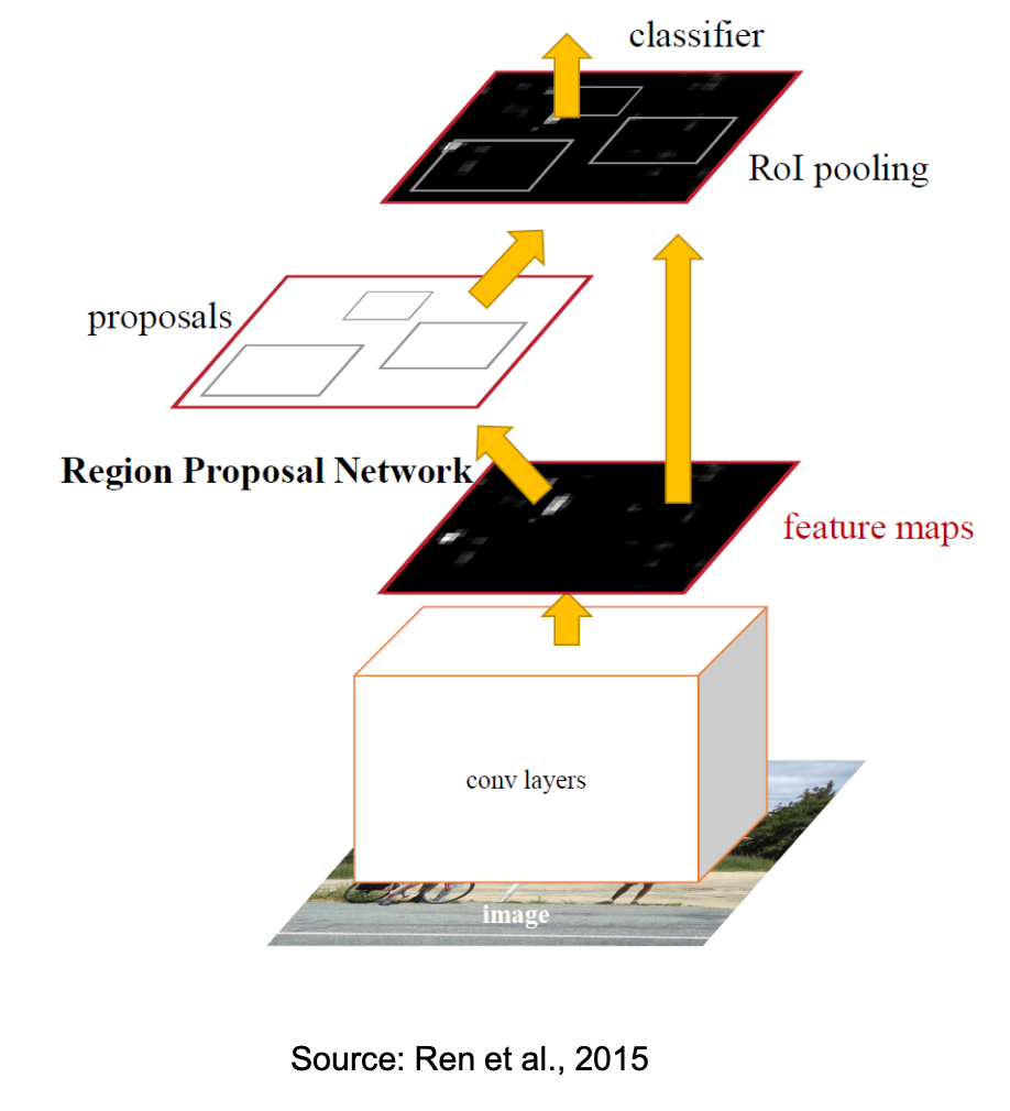
How to unify such features and make the Region Proposal Network take another image of a different size and run the classifier on that? i.e. handle variable-size inputs and still run a fixed classifier?

ROI Pooling or ROI Align. Once every ROI is a fixed size we want, they all look the same to the classifier — the size problem is gone.

Together with feature pyramids which handle scale variance, together they let one classifier handle any proposal from any image size.

How to get the proposals: the CNN extracts the features from the input image. Nowadays they use pyramids archiecture (that’s how they detect even small objects, they are able to adapt). The idea: a small network slides over a conv. feature map that is the output by the last conv. layer.

ROI (Region of Interest) is a proposed region from the original image. For ROI pooling, we approximate the new values by integers (always round down) i.e. quantization of coordinates on the feature map. However, we lose a bunch of data (the dark blue rectangle from the slide), yet we gain new data (the small green rectange).

A smarter solution though — ROI align: divide the original ROI into 9 equal size boxes and applying bilinear interpolation inside every one of them. This way, we don’t need to find narrow or expand the ROI, and use the float values directly.

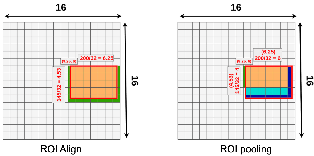
Reminder of max pooling: If you have multiple values in a 2x2 grid, then you take the largest one and discard the others. So the slide where I see 4 dots in each rectangle, I always select the highest value and store it in the final 3x3 ROIAlign result.

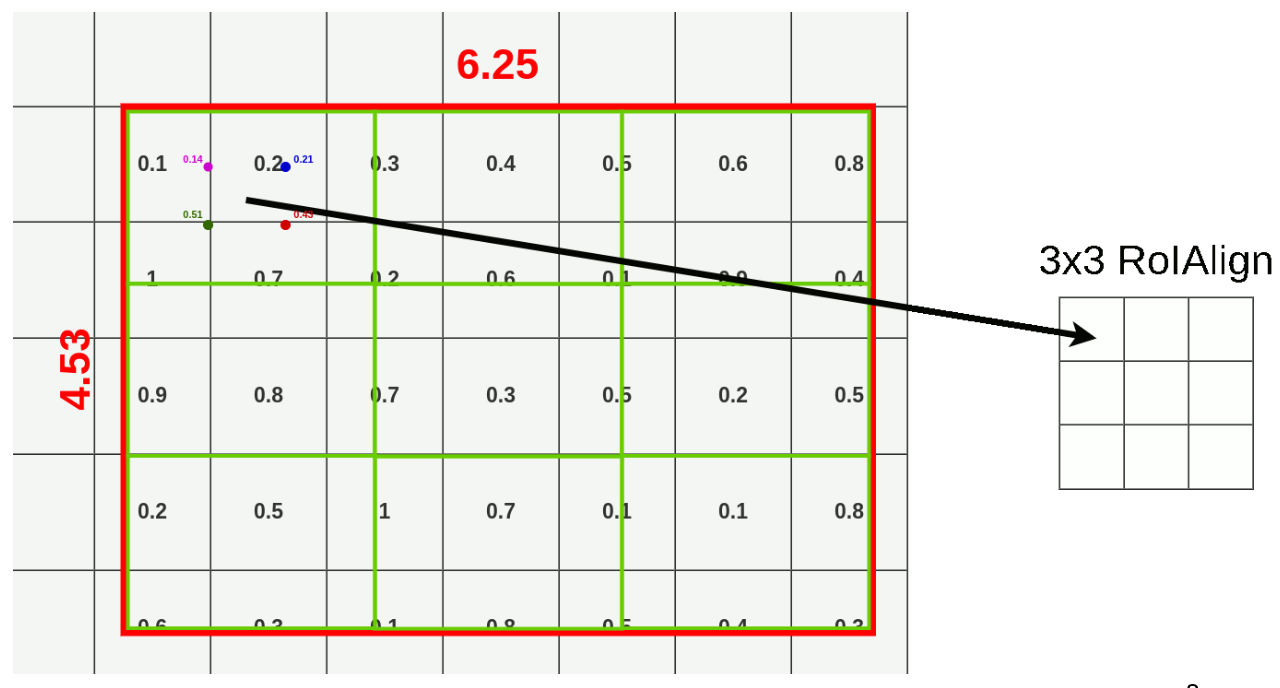
ROI Align is better usually per Hao’s words.

One stage Detectors

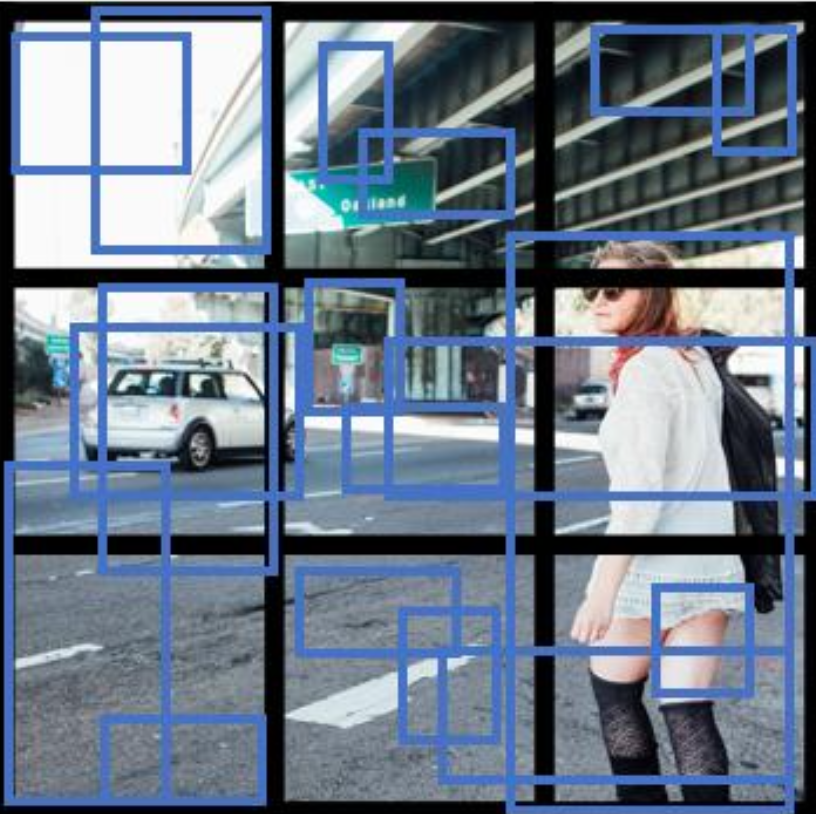
Of course, YOLO (You only look once). It uses a single CNN network for both classification and localizing the object using bounding boxes. The input image is divided into $3\times 3$ grid cells. it has great speed — main advantage.

Formulating the process: Instead of proposing regions first, you divide the image into a grid (here 3×3) and every cell simultaneously predicts: is there an object here + where is it + what is it? One forward pass, done.

• If Y is $1\times 8$ vector for 3 classes: [prob, bbx, bby, bbh, bbw, class1, class2, class3]
  • $100\times 100\times 3$ image ⇒ conv layers ⇒ $3\times 3\times 8$ output, one 8-dim vector per cell
    • The conv layers progressively downsample the spatial dimensions while outputting 8 channels at the end: 100x100x3 => 50x50x16 => 25x25x32 => 3x3x8
  • The exact architecture doesn’t matter — what matters is that you design the network so the final output is exactly grid_size x grid_size x (vector_size). This is corresponding to 9 cell results.

What if a gird cell wants to detect multiple objects?

We can extend Y with the two anchor boxes ⇒ Y will be $1\times 16$.

In the end, the process involves

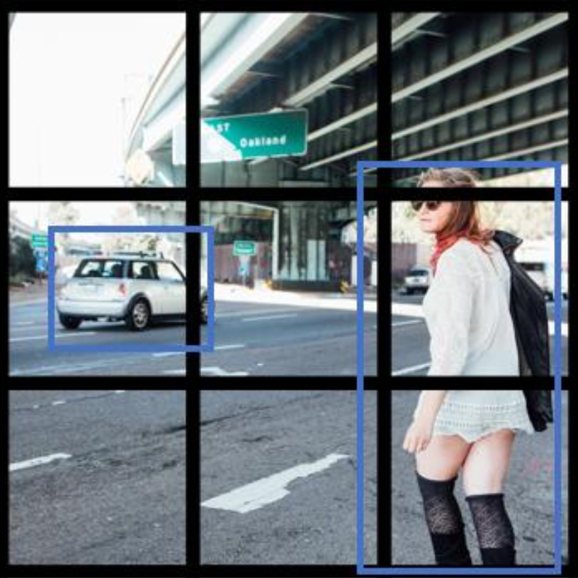
1. ConvNet + NMS
2. Removing the low probability predictions
3. Get the best probability by the IOU filtering

Object Tracking

Fundamentals of Object Tracking

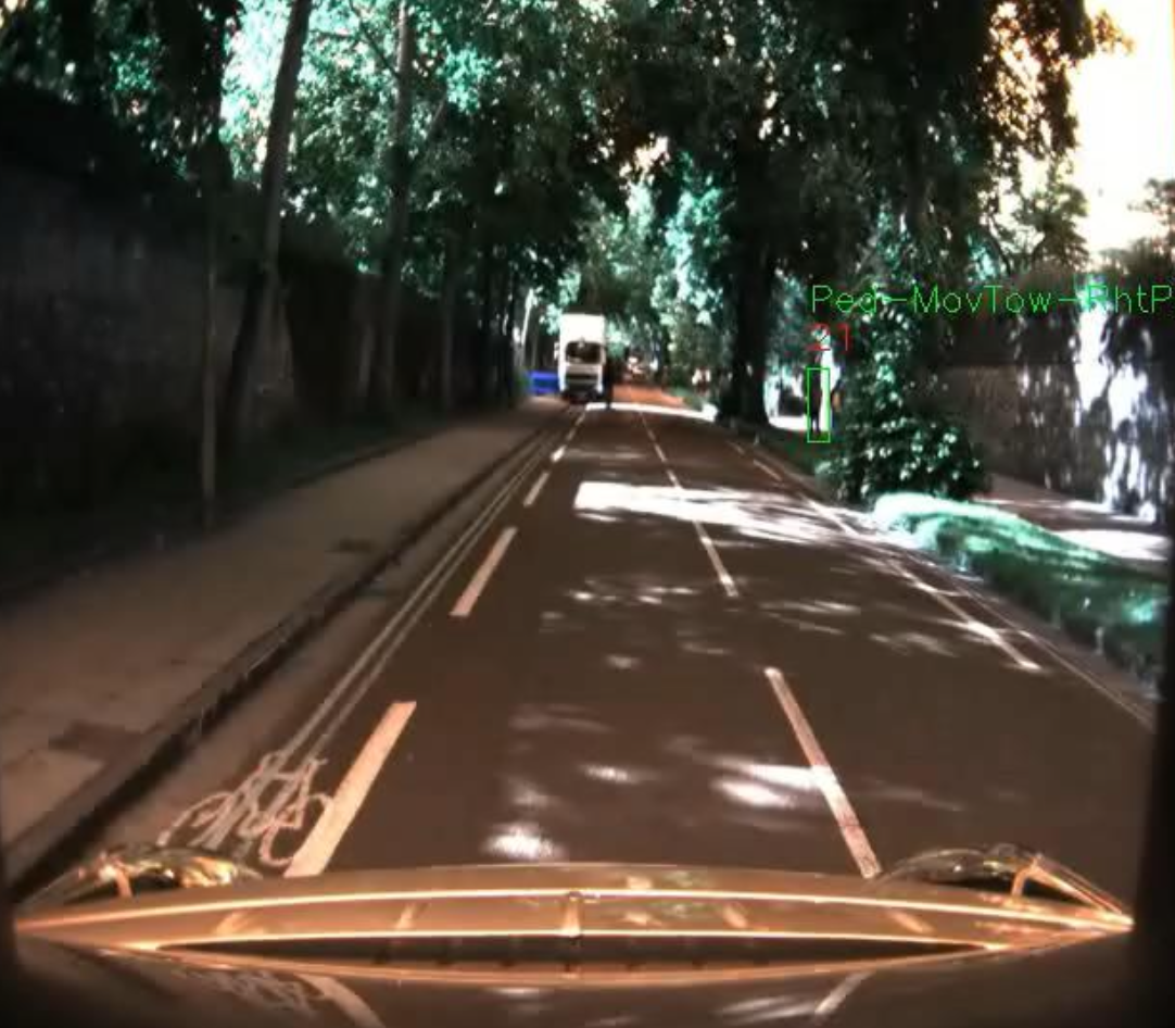
Object tracking is

continuously locating the target object across a sequence of images or video frames.

Some traditional methods include:

• Optical Flow (Lucas-Kanade / Farneback):
  • Assumes small motion between frames — breaks with fast movement
  • Assumes constant brightness — fails with lighting changes
• Kalman Filter:
  • Assumes linear motion — struggles with sudden direction changes
  • Needs a good initial state/model; if that’s wrong, it diverges
  • No appearance information — can’t re-identify an object if lost
• Mean-Shift:
  • Tracks by color histogram — fails if background has similar colors to the object
  • Fixed window size — doesn’t handle scale changes well (object getting closer/farther)
  • No notion of identity — if two similar-colored objects cross, it gets confused

Evaluation Metrics include: MOTA (Multi-Object Tracking Accuracy), Identity Preservation, HOTA (Higher Order Tracking Accuracy), Association Accuracy (measures how well the predicted identity matches the ground truth identity over time for that specific pair.)

Object Tracking Network Architectures

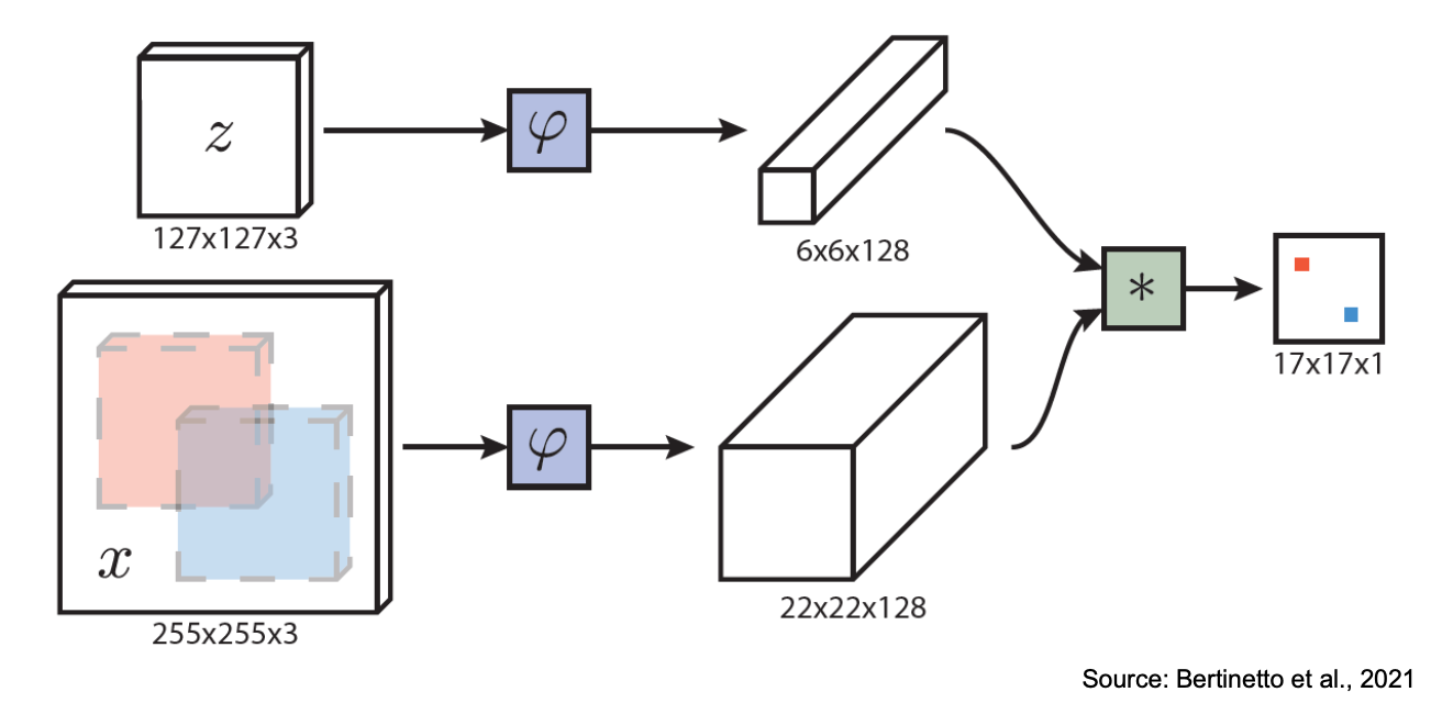
Siamese Networks — SiamFC

Track an object given only its initial bounding box (template)

• Template branch — $z(127\times 127\times 3)$: cropped from the first frame around the object.
• Search branch — $x(255\times 255\times 3)$: the larger search region from the current frame.
• Both pass through the same $\phi$ (shared weights, hence “Siamese”) ⇒ feature maps of $6\times 6\times 128$ and $22\times 22\times 128$.
• Cross-correlation (*) slides the template features over the search features ⇒ $17\times 17\times 1$ score map, where the peak tells you where the object is. Essentially a heatmap — the brightest point = most likely object location.

Multi-Object Tracking — DeepSORT

Instead of matching by similarity like SiamFC, it:

1. Detects objects each frame using YOLO.
2. Predicts where each tracked object should be next (Kalman).
3. Matches predictions to detections using both motion similarity (Mahalanobis Distance) and appearance similarity (Cosine distance).
4. Hungarian algorithm solves the optimal assignment.

In Track Management, we want to know whether the object appears constantly during consecutive frames.

Hungarian Assignment

Assigning new detections to existing tracks by finding the best possible matches while minimizing a cost metric.

• IoU distance, e.g. L_IoU = 1 - IoU
• Mahalanobis distance
• Appearance similarity.

As a problem definition, given:

• Detections: $D=\{d_1,d_2,\dots ,d_m\}$
• Tracks: $T=\{t_1,t_2,\dots ,t_n\}$
• Minimize cost matrix $C$ where $c_{ij}$ is the cost for assigning $d_j$ to $t_j$.

The Hungarian Assignment solves the optimization problem of assigning each track a detection.

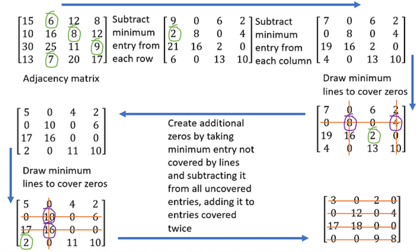
1. build the cost matrix: Each cell c_ij = cost of assigning detection i to track j (e.g. 1 - IoU).
2. subtract minimum entry from each row — guarantees at least one zero per row. Zeros = potential assignments.
3. same for the columns
4. draw minimum lines to cover all zeros. If the number of lines == matrix size ⇒ you have a valid assignment, done. If not, continue.
5. create additional zeros by taking minimum entry not covered by lines and subtracting it from all uncovered entries (see the encircled 2). Then you repeat steps 4 and 5 until you can cover all zeros with N lines.

What do we do if we have more detection than tracks or vice-versa?

We insert dummy entries. After the assignment, matches with dummy tracks will be unassigned detections and vice-versa.