Flow Matching and Mean Flows

Lecture from the GenAI Models and Robotic Applications. Related to Normalizing Flows.

Resources: Flow Matching for Generative Modeling paper, this blog from Cambridge

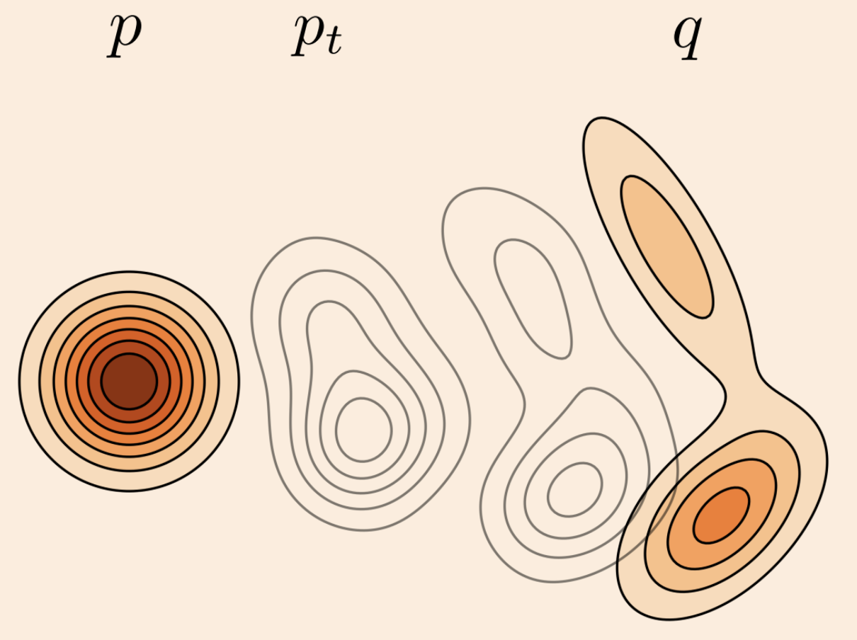
Flow matching is a training method used to learn a mapping from a source distribution to a target distribution by approximating the underlying vector field.

Diffusion $\in$ Flow Matching $\in$ Generative Models

Velocity Fields and Continuous Normalizing Flows (CNF)

In NF, we had $\mathbf{x}=f(z)$ and $\mathbf{x}=f_K\circ f_{K-1}\circ ...\circ f_1(z)$. The transformations are independent.

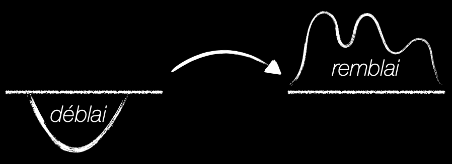
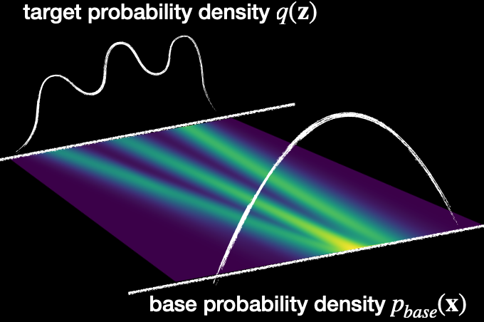
• Deblai: base probability density (to sample from)
• Remblai: target probability density (images, videos).

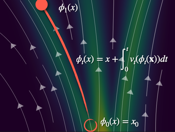
Time-Dependent Velocity Field

We have a trajectory from the noise to a realistic output ${\varphi }_0(\mathbf{x})={\mathbf{x}}_0$ …

Different definitions use different steps. We use $t=0\to t=1$.

We can now consider the rate of displacement in time with help of derivatives.

$$\frac{d}{dt}{\varphi }_t(x)=v_t(\varphi (x))$$

The velocity is essentially a model that given an input, time step, and parameter, it’s able to approximate the velocity with a neural network.

$$f(x,t,\theta )=v_t({\theta }_t(x))$$

We have a ordinary differential equation (ODE).

$$v_t(\varphi (x))=\frac{d}{dt}{\varphi }_t(x)$$ $$f_t(x)=\frac{dx}{dt}$$

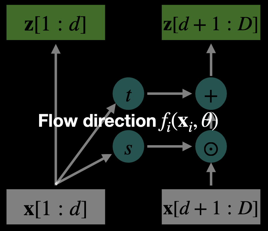
Which velocity fields are relevant?

We already covered in Normalizing Flows that with the help of Change-of-Variable Formula we can go from one Density Function to another with the following formula:

$$p_{base}({\mathbf{x}}^{\prime })=q({\mathbf{z}}^{\prime })\left|det[J_{\varphi }]\right|$$

• which is the same as

$$q(z^{\prime })=p_{base}({\mathbf{x}}^{\prime })\left|det[J_{{\varphi }^{-1}}]\right|$$

• where training is done via Maximum Likelihood Estimation

$$\log q(\mathbf{z})=\log p_{base}(\mathbf{x})+\log \left|det[J_{{\varphi }^{-1}}]\right|$$

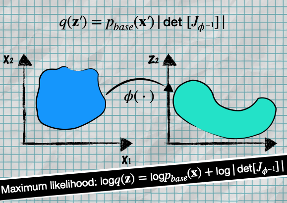
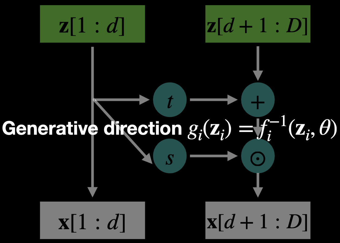
• don’t forget that to go from target distribution space $\mathbf{x}$ to latent space $\mathbf{z}$, we define $\mathbf{x}={\varphi }^{-1}(z)$

The logarithmic compression of a volume element equals the time-integrated expansion rate along its path

Jacobi’s formula

At this moment, we have complexity $O(n^2)$ because the Jacobian Matrix $J$ has $n\times n$ elements. If we want to compute the determinant of that, we actually have $O(n^3)$ complexity.

So using Jacobi’s formula, we show that we only need the Trace of the Jacobian Matrix (sum of the diagonal)

$$\left|\det [J_{{\varphi }^{-1}}]\right|=\left|\det \left[\begin{array}{cccc}\frac{\partial x_1}{\partial z_1}& \frac{\partial x_1}{\partial z_2}& \cdots & \frac{\partial x_1}{\partial z_n}\\ \frac{\partial x_2}{\partial z_1}& \frac{\partial x_2}{\partial z_2}& \cdots & \frac{\partial x_2}{\partial z_n}\\ ⋮& ⋮& \ddots & ⋮\\ \frac{\partial x_n}{\partial z_1}& \frac{\partial x_n}{\partial z_2}& \cdots & \frac{\partial x_n}{\partial z_n}\end{array}\right]\right|$$ $$\log \left|\det [J_{{\varphi }^{-1}}]\right|=-{\int }_0^1\text{Tr}\left(\frac{\partial {\mathbf{v}}_t({\varphi }_t(\mathbf{x}))}{\partial {\varphi }_t(\mathbf{x})}\right)dt$$

This reduces the complexity from $O(n^2)$ to $O(n)$.

So now, considering the equations from before, we can express the end location as the start $+$ the accumulated displacement over $t=\{0,1\}$:

$$\log q({\varphi }_1(\mathbf{x}))=\log p_{base}({\varphi }_0(\mathbf{z}))+{\int }_0^1\text{Tr}\left(\frac{\partial {\mathbf{v}}_t({\varphi }_t(\mathbf{x}))}{\partial {\varphi }_t(\mathbf{x})}\right)dt$$ $${\varphi }_1(\mathbf{x})=\mathbf{x}+{\int }_{t=0}^1{\mathbf{v}}_t({\varphi }_t(\mathbf{x}))dt$$

ODE numerical simulations are very expensive

Since we want to train a ODE NN with max likelihood. This is where Euler’s Method comes in.

For ordinary differential equations (ODEs) we can approximate their solution by taking small sequential steps using a tangent

Euler’s Method

$$\mathbf{x}={\mathbf{x}}_0+f_{t=0}({\mathbf{x}}_0)(t-t_0)$$

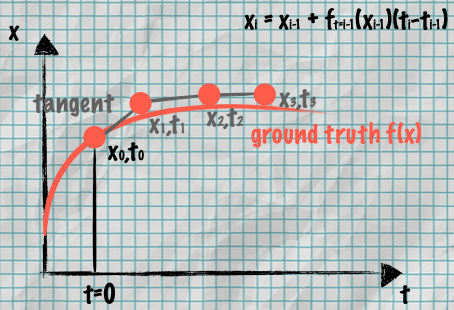
So I hope it’s clear that we approximate the velocity field with an ODE solver (e.g. Euler’s rule).

Now we can define the Loss Function of Flow Matching based models which is based on MSE (Mean Squared Error):

$${\mathcal{L}}_{FM}(\theta )=E_{t,p_t(\mathbf{x})}\left||{\mathbf{v}}_{\mathbf{t}}(\mathbf{x};\theta )-{\mathbf{u}}_{\mathbf{t}}(\mathbf{x})\right|{|}^2$$

where

• $p_t(\mathbf{x})$ is the probability path
• ${\mathbf{v}}_{\mathbf{t}}(\mathbf{x};\theta )$ is the velocity NN with $\theta$ params
• $u_t(\mathbf{x})$ is the velocity field from solver (Euler)

So I covered the fact that CNFs are slow due to the ODE integration at each iteration. CFMs are a very nice solution!

(Conditional) Flow Matching (CFM)

Can be CLIP as the condition(the label). They use the Euler approximation which gives those cartoonish effects in most generative models’ output. So it’s basically always sampling through an enormous database (400 million) in case of CLIP.

But what should the probability path be?

$$p_t(\mathbf{x})=\int p_t(\mathbf{x}\mid {\mathbf{x}}_1)d{\mathbf{x}}_1$$

The CFM loss function learns a velocity field conditioned on target samples ${\mathbf{x}}_1$ from $q({\mathbf{x}}_1)$, where $p_t(\mathbf{x}\mid {\mathbf{x}}_1)$ is a path distribution.

The key difference: CFM conditions on individual data points ${\mathbf{x}}_1$ from the target distribution $q({\mathbf{x}}_1)$, making training easier by decomposing the problem into simpler conditional paths.

$${\mathcal{L}}_{\text{CFM}}(\theta )={\mathbb{E}}_{t,q({\mathbf{x}}_1),p_t(\mathbf{x}|{\mathbf{x}}_1)}||{\mathbf{v}}_t(\mathbf{x};\theta )-{\mathbf{u}}_t(\mathbf{x}|{\mathbf{x}}_1)|{|}^2$$

• ${\mathbf{x}}_1$ is the image in the database
• ${\mathbf{x}}_0$ is the noise sample.
• c is the constraint from CLIP (text) or any other VLM.

CFM inference: find a image in the database based on the constraint (c = labels(i)).

• Key Insights:
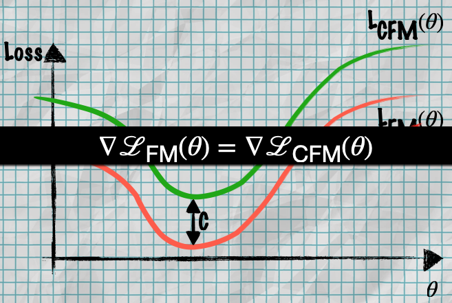
• Their gradients are identical. The two loss functions only differ by a constant offset C
• Optimizing CFMs is equivalent to optimizing FMs (same optimal parameters)
• So you can train using CFM and get the same results as the harder-to-compute FM

Reminder: velocity is the rate of change between random noise and the image from the database.

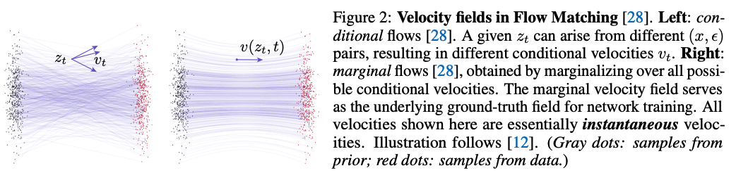
You use the conditional flows to define your loss function (left) during training, but what emerges from that training is a network that predicts the marginal flow(right).

Conditional flows are the individual velocity fields for specific conditioning pairs $(\mathbf{x},ϵ)$. They are used to construct the training objective but aren’t directly what the network predicts.

Marginal flows are what you get when you average all those conditional flows together. This is the actual velocity field the network learns to predict.

Mean Flows

Resource: Mean Flows for One-step Generative Modeling

Code implementation: this blog

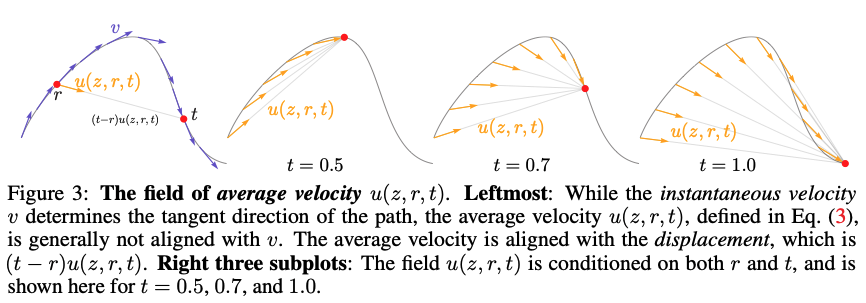
The core idea is to introduce a new ground-truth field representing the average velocity $\bar{v}$, whereas the velocity modeled in Flow Matching represents the instantaneous velocity $v$.

Flow Matching essentially models the expectation over all possibilities, called the marginal velocity $v({\mathbf{z}}_t,t)={\mathbb{E}}_{{\rho }_t(v_t|{\mathbf{z}}_t)}[v_t]$ given a marginal velocity field $\frac{d}{dt}{\mathbf{z}}_t=v({\mathbf{z}}_t,t)$

Given the actual data $\mathbf{x}\sim p_{data}(\mathbf{x})$ and the noise $ϵ\sim p_{prior}(ϵ)$, a flow path can be constructed as ${\mathbf{z}}_t=t\mathbf{x}+(1-t)ϵ$

$${\bar{v}}_t({\mathbf{z}}_t,t,r)=\frac{1}{t-r}{\int }_r^{t}v({\mathbf{z}}_{\tau },\tau )d\tau$$

By setting $r=0$ and $t=1$, we can instantly generate outputs from inputs (1-step only). So the “core idea” is we can generate with less steps, since the model already averages over $r,t$. If $r=t$, then it reduces to standard Flow Matching.

The bigger the step, much farther away we are from the actual image. I want to not be constrained by where I am. I want to start at r and stop at t. I’ll take the average velocity accumulated. $\tau =t-r$ is the new timestep. It works best for bigger steps.

The ultimate aim will be to approximate the average velocity using a neural network $\bar{v}({\mathbf{z}}_t,t,r,\theta )$. The approach is much more amenable to single or few-step generation, as it does not need to explicitly approximate a time integral at inference time, which was required when modeling instantaneous velocity.

Mean Flow Training

The Mean Flow Identity:

$$(t-r)\bar{v}({\mathbf{z}}_t,r,t)={\int }_r^{t}v({\mathbf{z}}_t,\tau )d\tau$$ $$\frac{d}{dt}(t-r)\bar{v}({\mathbf{z}}_t,r,t)=\frac{d}{dt}{\int }_r^{t}v({\mathbf{z}}_t,\tau )d\tau$$ $$\frac{d}{dt}(t-r)\bar{v}({\mathbf{z}}_t,r,t)=v({\mathbf{z}}_t,t)$$ $$(t-r)\frac{d}{dt}\bar{v}({\mathbf{z}}_t,r,t)+\bar{v}({\mathbf{z}}_t,r,t)=v({\mathbf{z}}_t,t)$$

And therefore we can finally express the average velocity as:

$$\bar{v}({\mathbf{z}}_t,r,t)=v({\mathbf{z}}_t,t)-(t-r)\frac{d}{dt}\bar{v}({\mathbf{z}}_t,r,t)$$

Training with Average Velocity:

We now introduce a model $\bar{v}({\mathbf{z}}_t,r,t,\theta )$ to learn $\bar{v}({\mathbf{z}}_t,r,t)$ (denoted as ${\bar{v}}_{tgt}$)

And in the end, the loss function for Mean Flow models is represented as

$${\mathcal{L}}_{MF}(\theta )=\mathbb{E}\left||\bar{v}({\mathbf{z}}_t,r,t,\theta )-sg({\bar{v}}_{tgt})\right|{|}_2^2$$

From the paper: The term ${\bar{v}}_{tgt}$ uses the instantaneous velocity $v$ as the only ground-truth signal; no integral computation is needed. While the target should involve derivatives of $\bar{v}$ ($\partial \bar{v}$), they are replaced by their parametrized counterparts ($\partial {\bar{v}}_{\theta })$. In the loss function, a stop-gradient (sg) operation is applied on the target because it eliminates the need for “double backpropagation” through the Jacobian-vector product, thereby avoiding higher-order optimization.

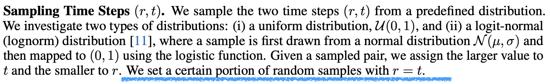
The loss function is as in FM, but they take the mean velocity. Understand the highlighted part from the paper ($t=r$). You mix the mean flow and the normal flow (In some steps you do one, in some you do the other). I mentioned above that if $r=t$, then it reduces to standard Flow Matching.