Point Cloud Segmentation with Segment Anything (SAM)

We will use Segment Anything (SAM) from META. I also used it in Visual-Language Models for Object Detection and Segmentation. Again, I can see the similarity between image processing and point cloud segmentation. So basically the previous topic Point Cloud Segmentation applied the segmentation techniques in directly in the 3D unordered space of point clouds, and this one applies segmentation in the projected 2D space using deep NNs.

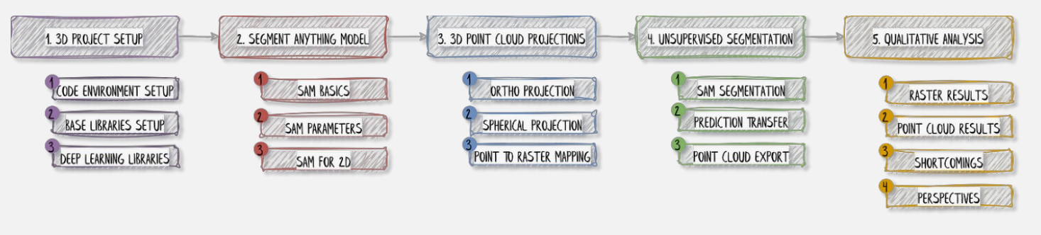
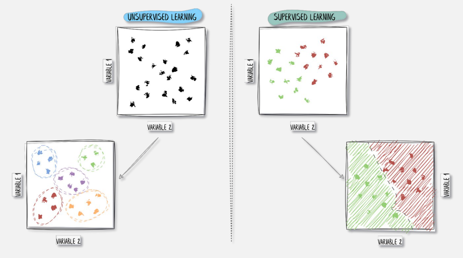
Unsupervised segmentation enters the scene, in the form of the Segment Anything Model (SAM). We are, in the case of non-labeled outputs, through SAM’s segmentation architecture. This is opposed to the supervised learning approach where we do have labels.

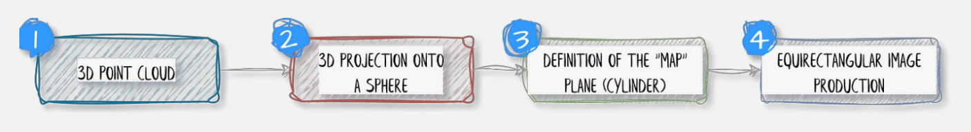
Projection from 3D to 2D

Projecting from 3D to 2D is primarily done to convert unstructured point cloud data into a structured grid format that can be processed by standard computer vision tools. While raw point clouds are difficult to analyze because they lack a fixed neighborhood structure, a 2D projection behaves like a digital image where spatial relationships are defined by pixel positions. This allows me to leverage highly optimized deep learning architectures, such as CNNs, which excel at identifying patterns in regular grids.

• (ortho) Normal projection i.e. setting a plane direction and/or orthogonal projection direction.
  • Mostly for parallel views. We ignore Z.
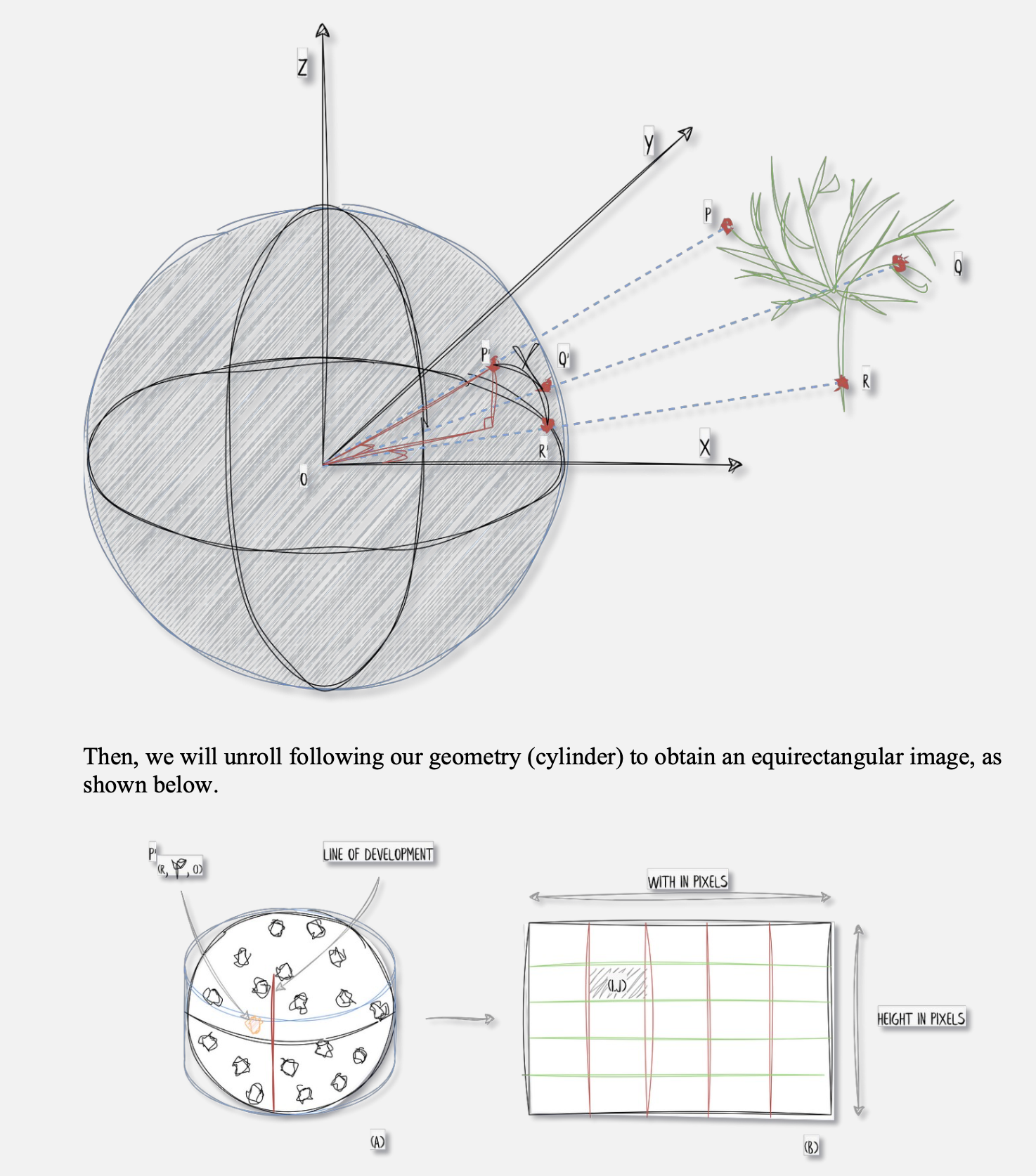
• Spherical/Cylindrical projection
  • Set a center location
  • generate an artificial sphere/cylinder
  • project point cloud onto the cylinder/sphere (intersection between each point and center point)
• Perspective projection using a camera’s intrinsics and extrinsics
  • Not based on features, look into it.

What kind of information do I project?

• Color
• Height
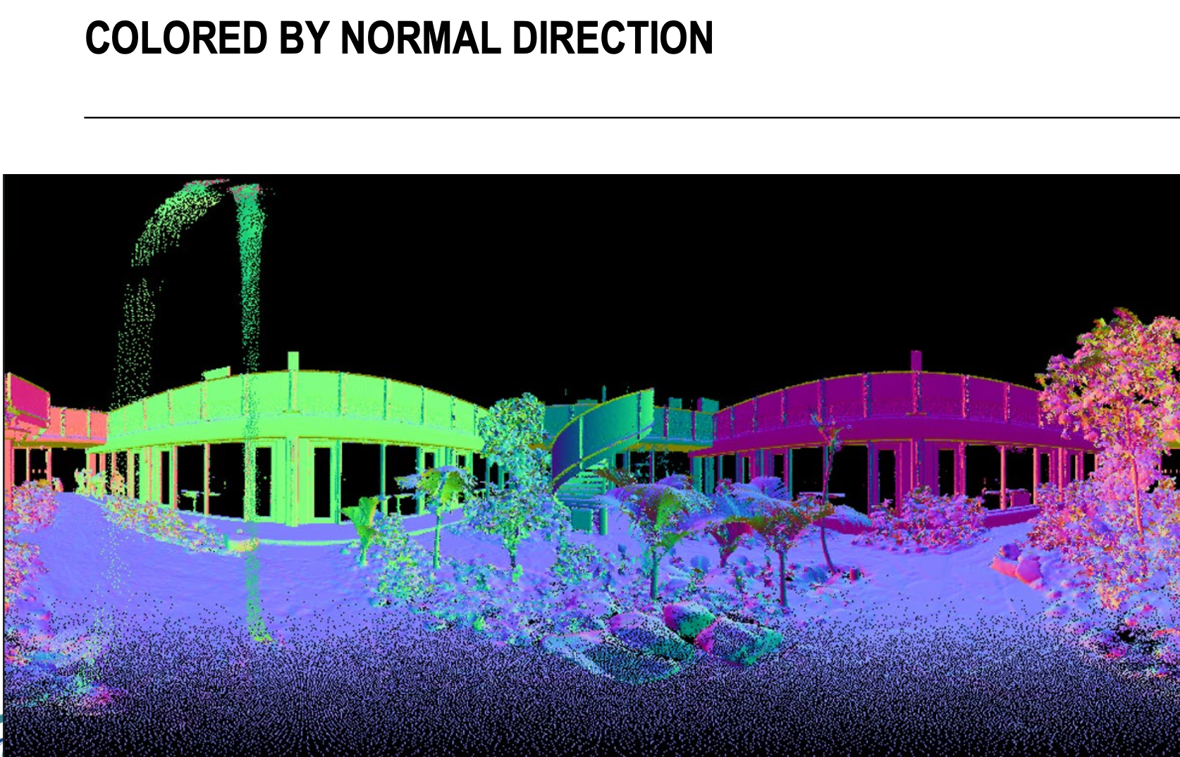
• Normal

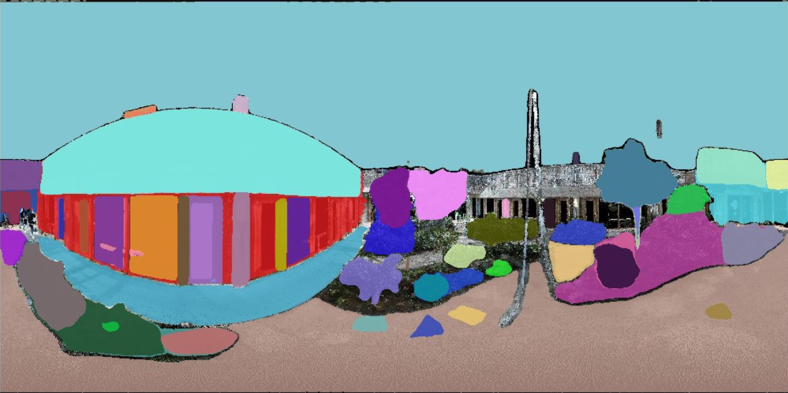
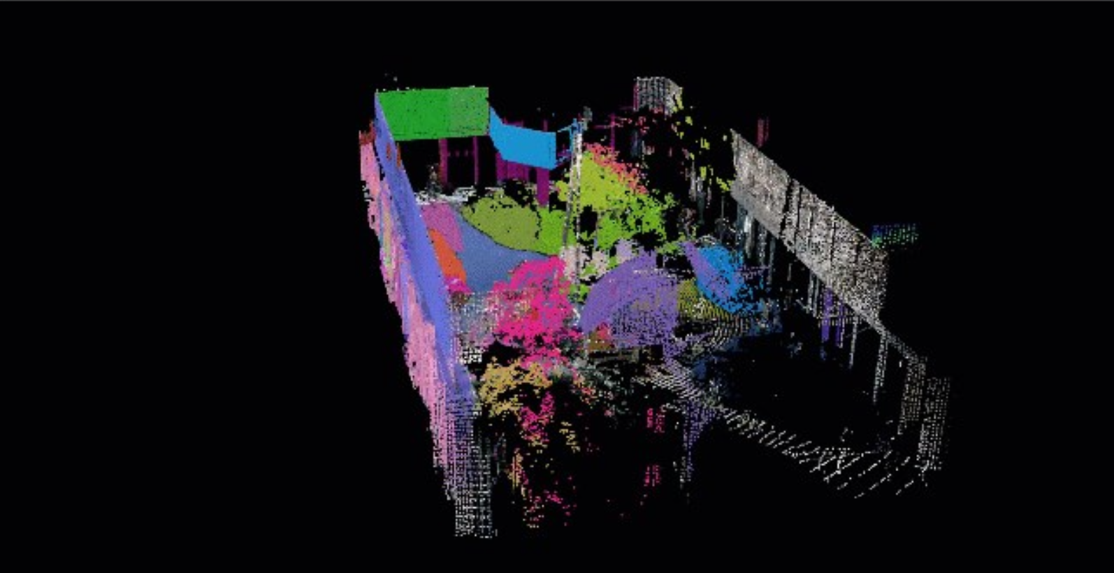
SAM is applied on the image ⇒ automatic segmentation based on given number of input prompts (in our case a regular grid of point of interest).

Gemini: Meta's Segment Anything Model (SAM) is fundamentally a 2D image-based model, meaning it cannot process raw 3D point clouds directly. To use SAM for 3D data, you have to follow the exact workflow described in your slides: you project the 3D points into one or more 2D images, run SAM to segment those images, and then map the resulting 2D masks back onto the original 3D points.

Why are there multiple ways of projecting the point cloud?

Essentially, you must pick the projection that minimizes distortion for your specific viewpoint; aerial data needs a flat map-like grid to keep building shapes consistent, while a 360 degrees scanner needs a wrap-around view to ensure nearby objects aren’t squashed into a single line of pixels.

• If you apply a normal projection to data collected from a ground-based scanner, points further from the sensor become extremely sparse and stretched, which prevents a model like SAM from recognizing objects accurately. Spherical projection is better for sensors on cars or robots because it mimics the scanner’s circular “sight,” maintaining consistent data density even if it curves straight lines.

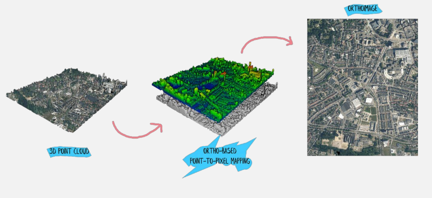
Ortho Projection: Flattening Dimensions, Expanding Insights

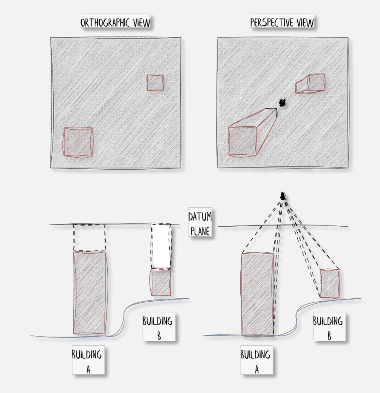
The idea is basically to generate a top-down view plane and generate an image that is not constrained by a single perspective. You could see ortho-projection as a process of pushing visible points from the point cloud (highest ones) onto the plane that holds the empty image to fill all the necessary pixels just above those points.

This permits us to obtain the following (keep in mind, ignore Z).

def cloud_to_image(pcd_np, resolution):
 
	minx = np.min(pcd_np[:, 0])
	maxx = np.max(pcd_np[:, 0])
	miny = np.min(pcd_np[:, 1])
	maxy = np.max(pcd_np[:, 1])
	width = int((maxx - minx) / resolution) + 1
	height = int((maxy - miny) / resolution) + 1
	image = np.zeros((height, width, 3), dtype=np.uint8)
 
	for point in pcd_np:
		x, y, *_ = point
		r, g, b = point[-3:]
		pixel_x = int((x - minx) / resolution)
		pixel_y = int((maxy - y) / resolution)
		image[pixel_y, pixel_x] = [r, g, b]
 
	return image

3D Point Cloud Spherical Projection

1. Project the point cloud onto a sphere
2. Defining a geometry that will retrieve the pixels
3. “Flattening” this geometry to produce an image

def generate_spherical_image(center_coordinates, point_cloud, colors, resolution_y=500):
	
	# Translate the point cloud by the negation of the center coordinates
	translated_points = point_cloud - center_coordinates
	
	# Convert 3D point cloud to spherical coordinates
	theta = np.arctan2(translated_points[:, 1], translated_points[:, 0])
	phi = np.arccos(translated_points[:, 2]/np.linalg.norm(translated_points, axis=1))
	
	# Map spherical coordinates to pixel coordinates
	x = (theta + np.pi) / (2 * np.pi) * (2 * resolution_y)
	y = phi / np.pi * resolution_y
	
	# Create the spherical image with RGB channels
	resolution_x = 2 * resolution_y
	image = np.zeros((resolution_y, resolution_x, 3), dtype=np.uint8)
	
	# Create the mapping between point cloud and image coordinates
	mapping = np.full((resolution_y, resolution_x), -1, dtype=int)
	
	# Assign points to the image pixels
	for i in range(len(translated_points)):
		ix = np.clip(int(x[i]), 0, resolution_x - 1)
		iy = np.clip(int(y[i]), 0, resolution_y - 1)
		if mapping[iy, ix] == -1 or np.linalg.norm(translated_points[i]) < np.linalg.norm(translated_points[mapping[iy, ix]]):
			mapping[iy, ix] = i
			image[iy, ix] = colors[i]
	
	return image, mapping

Reprojection of the points back to 3D

def color_point_cloud(image_path, point_cloud, mapping):
 
	image = cv2.imread(image_path)
	h, w = image.shape[:2]
	modified_point_cloud=np.zeros(
		(point_cloud.shape[0],point_cloud.shape[1]+3), 
		dtype=np.float32)
		
	modified_point_cloud[:, :3] = point_cloud
	for iy in range(h):
		for ix in range(w):
			point_index = mapping[iy, ix]
			if point_index != -1:
				color = image[iy, ix]
				modified_point_cloud[point_index, 3:] = color
	
	return modified_point_cloud

Shortcomings:

• all the “unseen” points remain unlabeled
• cannot tune the prompting engine, the automatic one was used which triggered around 50 points of interest.
• the mapping is somewhat simple at this stage; it would largely benefit from occlusion culling and point selection for a specific pixel of interest.