3D Point Cloud Shape Detection for Indoor Modeling

This is a practical side of 3D Indoor Reconstruction. The library used in these implementations is Open3D.

Point Clouds can be very big. Therefore, we sometimes want to reduce the size while preserving overall structural integrity and representativeness. I see they suggest Random Sampling for decimation of the point cloud. I think the same is applied in RandLA-Net?

• If we consider the point cloud a matrix ($m\times n$), the decimation acts by keeping points for every n-th row depending on the $n$ factor.

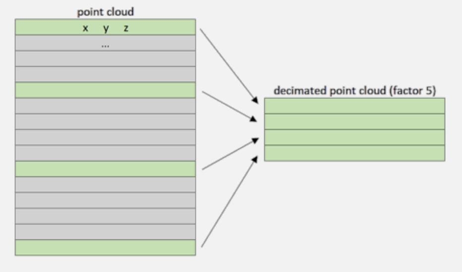
Needless to say, this method can go very wrong since we don’t know how important the dropped points might be.

The next step is statistical outlier removal which eliminates points that deviate from average neighborhood distances.

After removing statistical outliers from the point cloud, the next step involves applying voxel-based sampling techniques to downsample the data further.

Voxel Grid Sampling

The grid subsampling strategy is based on the division of the 3D space in regular cubic cells called voxels. For each cell of this grid, we only keep one representative point, and this point, the representative of the cell, can be chosen in different ways. When subsampling, we keep that cell’s closest point to the barycenter.

Point Cloud Normal Vectors Extraction

Important topic

A point cloud normal refers to the direction of a surface at a specific point in a 3D point cloud. It can be used for segmentation by dividing the point cloud into regions with similar normals, for example. It helps A LOT, since you can see which surfaces are perpendicular, it helps in dividing into vertical and horizontal, combining surfaces together.

• We first define the average distance between each point in the point cloud and its neighbors.
• Then we use this information to extract a limited number of points within a radius to compute a normal for each point in the 3D point cloud.
• George said the same thing. Pick close points and see what plane they define together. Do this for every point, since not all of those points should receive the same normal vector.

3D Shape detection and clustering

They cover RANSAC and Euclidean Clustering using DBSCAN.

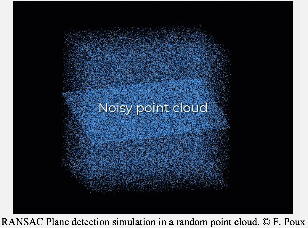
RANSAC

It works by randomly sampling minimum points to fit a plane, scoring the model based on how many other points fall within a distance threshold, and iterating to find the best fit. It is also very known for how well it handles outliers. By identifying and ignoring the outliers, you can focus on working with reliable inliers

The idea is very much similar to the normal vector above.

First, we create a plane from the data, and for this, we randomly select 3 points from the point cloud necessary to establish a plane. And then, we simply check how many of the remaining points kind of fall on the plane (to a certain threshold), which will give a score to the proposal.

• each iteration samples 3 random points from which it will create a plan and then select the points that would fall on it. Here, iteration 159 would be the best candidate.
• then, we repeat the process with 3 new random points and see how we are doing
• and then we select the plane model with the highest score

Determination of the Distance threshold

Ok so even RANSAC needs some parameters, and one of them is the minimum distance between two points to be considered in the same plane. Normally, the mean distance between points in the dataset should be good enough.

To determine such a value, we use a KD-Tree to speed up the process of querying the nearest neighbors for each point. From there, we can then query the k-nearest neighbors for each point in the point cloud,

Another parameter is the number of points, but it’s self-explanatory that at least 3 points define a 3D plane.

Scaling 3D Segmentation: Multi-Order RANSAC

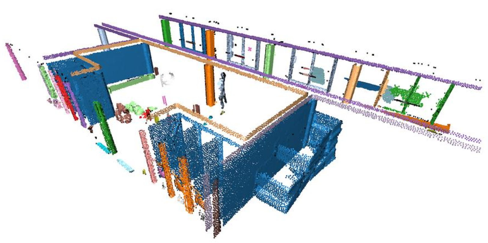
We will first run RANSAC multiple times (let’s say $n$ times) to extract the different planar regions constituting the scene. Then we will deal with the “floating elements” through Euclidean Clustering (DBSCAN). You can see below what they mean by “floating points”.

DBSCAN provides Euclidean clustering to refine the RANSAC outputs. Because RANSAC fits mathematical planes that stretch infinitely, DBSCAN groups only the spatially contiguous points based on local density to cleanly separate actual objects from artifacts.

rest=pcd
for i in range(max_plane_idx):
	colors = plt.get_cmap("tab20")(i)
	segment_models[i], inliers = rest.segment_plane(
	distance_threshold=0.1,ransac_n=3,num_iterations=1000)
	segments[i]=rest.select_by_index(inliers)
	segments[i].paint_uniform_color(list(colors[:3]))
	rest = rest.select_by_index(inliers, invert=True)
	print("pass",i,"/",max_plane_idx,"done.")

In the first pass, we separate the inliers from the outliers. We store the inliers in segments, and then we want to pursue with only the remaining points stored in rest, that becomes the subject of interest for the loop $n+1$ (loop $i=1$). That means that we want to consider the outliers from the previous step as the base point cloud until reaching the above threshold of iterations.

Euclidean Clustering (DEBSCAN)

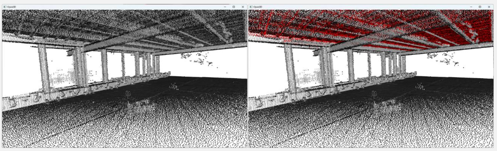
With point cloud datasets, we often need to group sets of points spatially contiguous (i.e. that are physically close or adjacent to each other in 3D space). The Figure below shows some “red lines/planes” that actually cut some planar elements. Because we fit all the points to RANSAC plane candidates (which have no limit extent in the Euclidean space) independently of the point’s density continuity, then we have these “lines” artifacts depending on the order in which the planes are detected.

Euclidean Clustering refines the inlier point sets in contiguous clusters.

DEBSCAN

The DBSCAN algorithm involves scanning through each point in the dataset and constructing a set of reachable points based on density. This is achieved by analyzing the neighborhood of each point and including it in the region if it contains enough points. The process is repeated for each neighboring point until the cluster can no longer expand. Points that do not have enough neighbors are labeled as noise, making the algorithm robust to outliers.

segments[i]=rest.select_by_index(inliers)
labels = np.array(segments[i].cluster_dbscan(eps=epsilon,
min_points=min_cluster_points))
candidates=[len(np.where(labels==j)[0]) for j in np.unique(labels)]
best_candidate=int(np.unique(labels)[np.where(candidates==np.max(candidates))[0]])
 
rest = rest.select_by_index(inliers, invert=True) + segments[i].select_by_index(list(np.where(labels!=best_candidate)[0]))
segments[i]=segments[i].select_by_index(list(np.where(labels==best_candidate)[0]))
""" the rest variable now makes sure to hold both the remaining points from RANSAC and DBSCAN. And of course, the inliers are now filtered to the biggest cluster present in the raw RANSAC inlier set.
 
When the loop is over, you get a clean set of segments holding spatially contiguous point sets that follow planar shapes, that you can visualize with different colors using the following lines of code in the loop
 """
colors = plt.get_cmap("tab20")(i)
segments[i].paint_uniform_color(list(colors[:3]))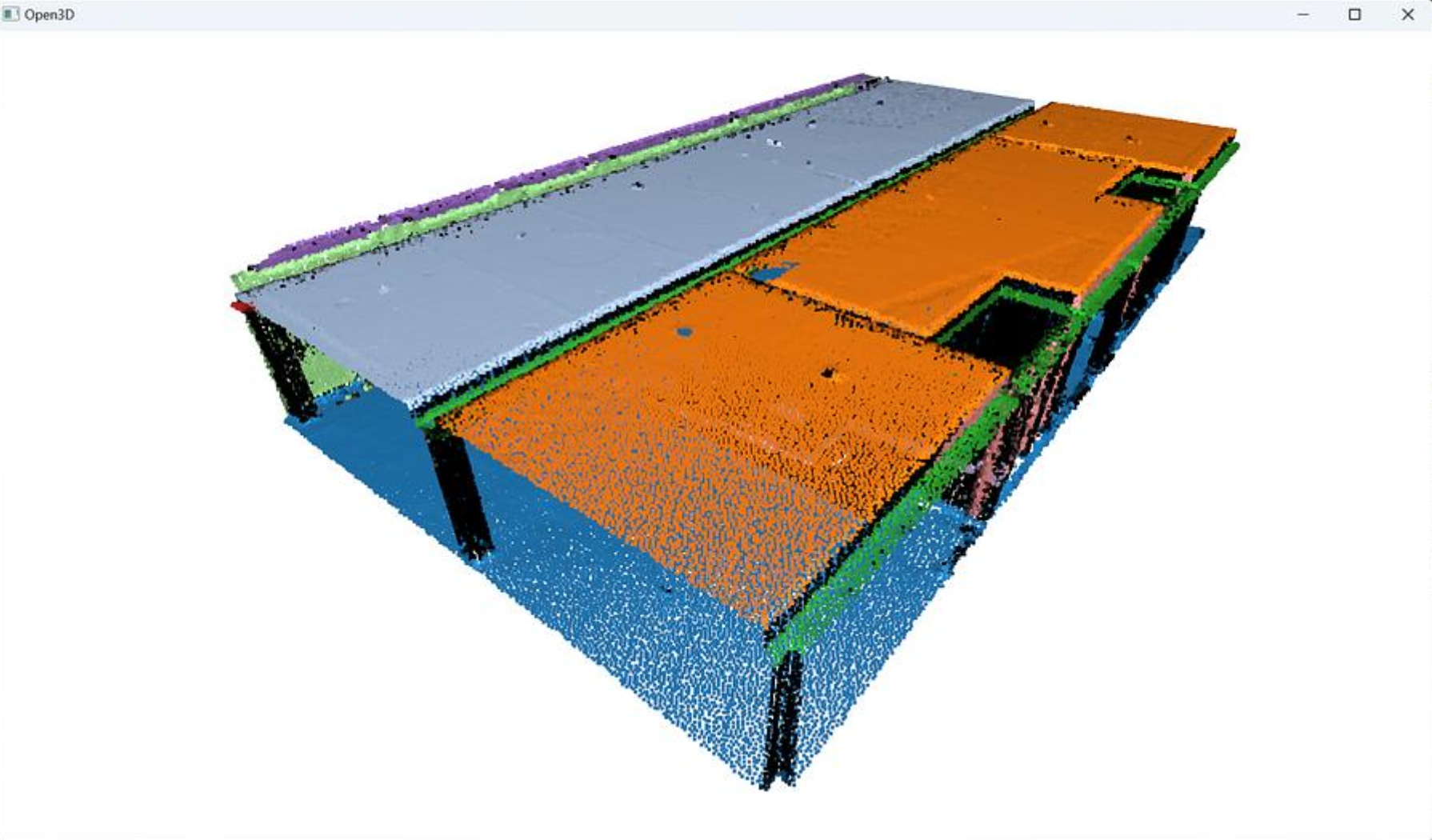

The next step involves working on the remaining points assigned to the rest variable, that are not yet attributed to any segment. We can apply a simple pass of Euclidean clustering with DBSCAN and capture the results in a labels variable.

labels = np.array(pcd.cluster_dbscan(eps=0.1, min_points=10))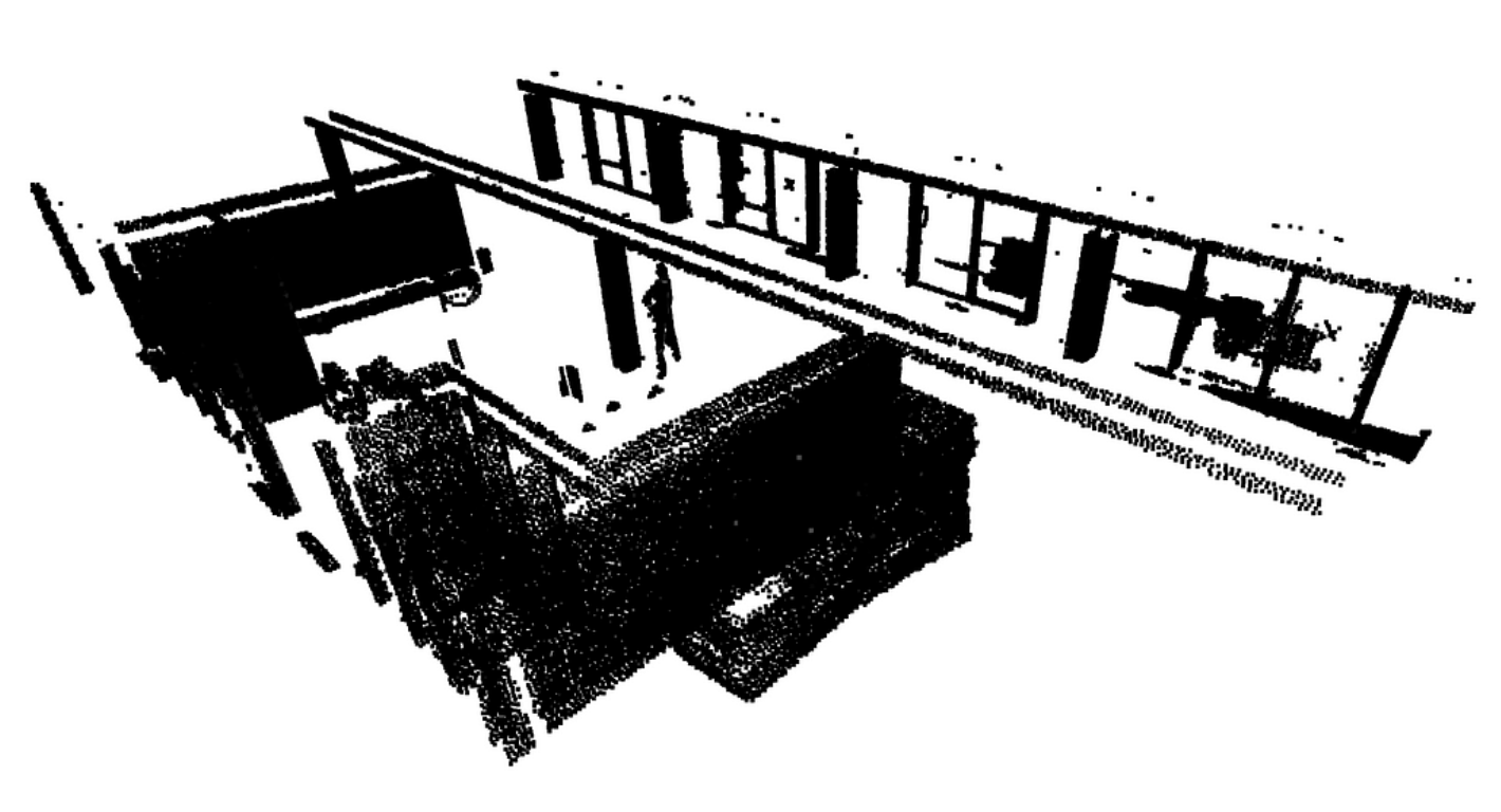

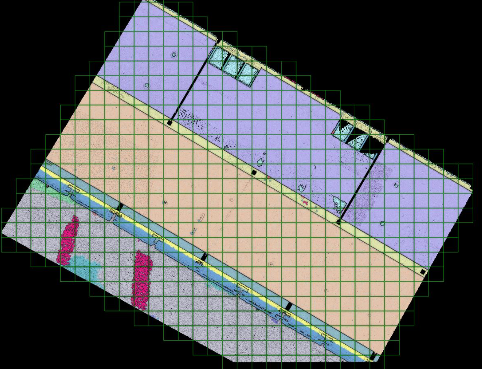
Voxelization

After refining the point cloud clustering results using DBSCAN, the focus shifts to the voxelization technique, which involves organizing the data into a meaningful spatial structure.

Voxelization translates the point data into a regular grid of cubes. This allows the algorithm to explicitly label structural elements, clutter, and empty navigable space for modeling applications.

This technique divides a point cloud into small cubes or voxels with their own coordinate system. Great for robots if they need to avoid collisions!

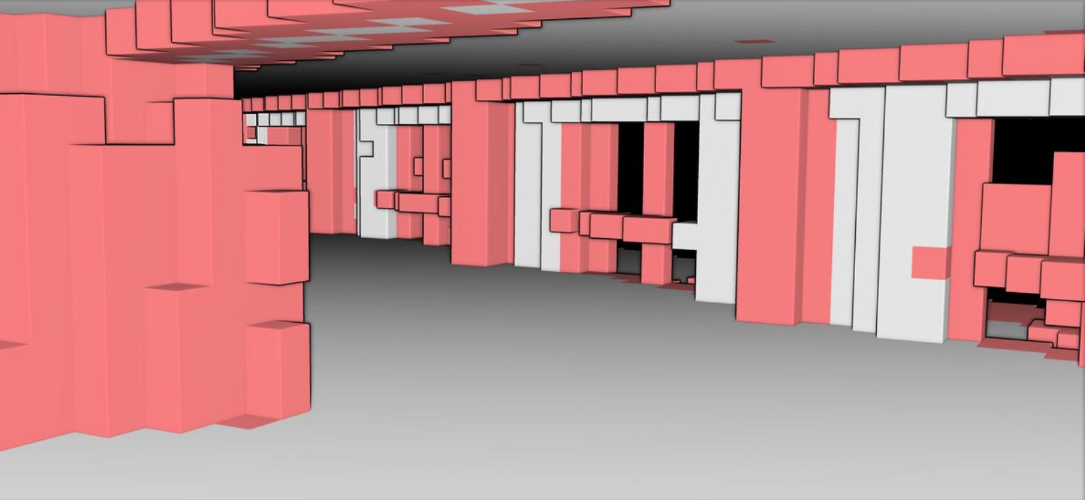
Now that we have a point cloud with segment labels, it would be very interesting to see if we could fit indoor modeling workflows (covered in 3D Indoor Reconstruction). One way to approach this is the use of voxels to accommodate for O-Space and R-Space. By dividing a point cloud into small cubes, it becomes easier to understand a model’s occupied and empty spaces.