Real-Time LiDAR Point-Cloud Moving Object Segmentation for Autonomous Driving

Link to research paper.

Context and adjacent research

As an abstract, autonomous driving should be able to recognize static and moving objects in the environment in order to avoid collisions and plan tasks (i.e. predicting the future state of the environment). To be able to perform real-time, they propose a lightweight MOS (Moving Object Segmentation) network structure based on LiDAR point-cloud sequence range images with only 2.3 M parameters, which was 66% less than the state-of-the-art network at that time.

RTX 3090TI GPU Performances:

• 35.82ms processing time per frame
• IoU score of 51.3% on the SemanticKITTI dataset.

On a custom FPGA, they reach 32fps, highly exceeding the standard of 10 fps regarding LiDAR navigation algorithms for real-time.

Autonomous Vehicles can already perform point-cloud pre-processing and neural network segmentation. Therefore, only post-processing is left for the ECU (Electronic Control Unit). This is where their contribution shines:

1. their implementation was one of the first end-to-end FPGA (ZCU104 MPSoC FPGA platform) implementations where a LiDAR is directly connected to the processing system (PS) side. After pre-processing, the point-cloud is stored in the DDR memory, which is accessible by the hardware accelerator on the programmable logic (PL) side
2. they made the implementation “hardware-friendly” by replacing deconvolution with bi-linear interpolation (look into it)

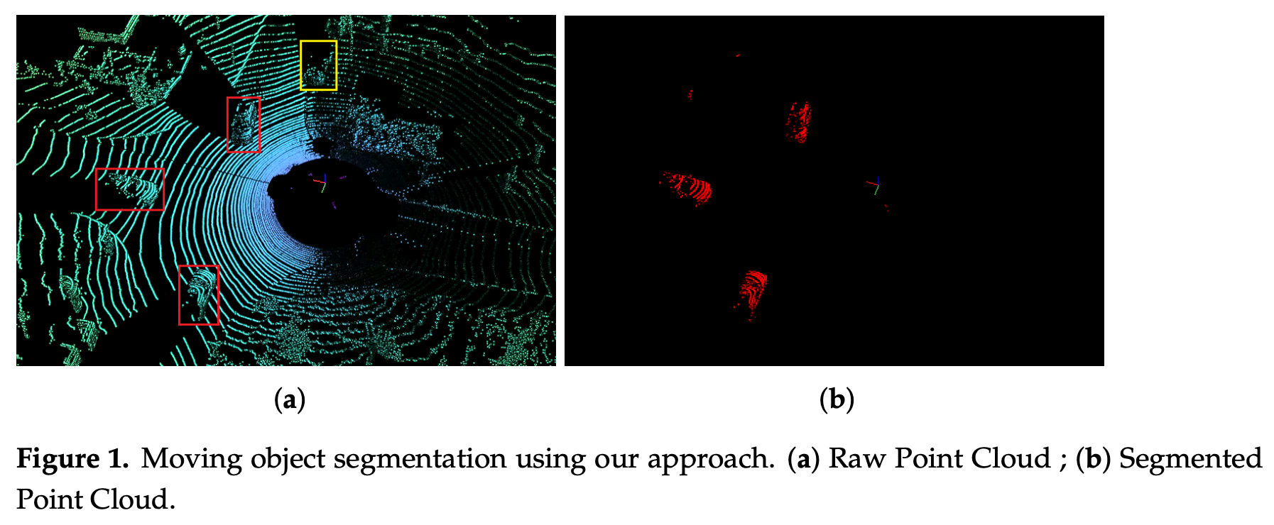
• Moving objects are represented by red masks.
• The yellow box is a parked car. So I assume yellow means stationary?
• Most of the existing architectures only predict semantic labels (vehicles, buildings, people), but cannot distinguish between moving and static objects as in this example.

Existing MOS networks really can be categorized into two groups:

1. computer-vision-based. Here I remember a paper from TNO where they fed consecutive frames to a CNN to detect small moving objects. Maybe similar to that.
2. LiDAR-sensor-based

However, it is the processing of LiDAR data that remains challenging due to the sparsity characteristic of point clouds.

One problem with all networks based on operating directly on the point cloud is the dramatic increase in processing power and memory requirements, causing the point cloud to become larger

LMNet utilizes the residual between the current frame and the previous frame as an additional input to the semantic segmentation network to achieve class-independent moving object segmentation. The same idea is adapted in RangeNet++ and SalsaNext for performance evaluation. In Efficient Spatial-Temporal Information Fusion for LiDAR-Based 3D Moving Object Segmentation, they utilize a dual-branch structure to fuse the spatio-temporal information of LiDAR scans to improve the performance of MOS.

Shifting towards attention-based architectures (check this info), EmPointMovSeg: Sparse Tensor Based Moving Object Segmentation in 3D LiDAR Point Clouds for Autonomous Driving Embedded System the autoregressive system identification (AR-SI) theory was used and it significantly improved the segmentation effect of the traditional encoder-decoder structure.

Why FPGAs? They provide high energy efficiency ratio and flexible reconfiguration. In Real-Time LiDAR Point Cloud Semantic Segmentation for Autonomous Driving, a LiDAR sensor is directly connected to FPGA through an Ethernet interface, realizing a deep learning platform of end-to-end 3D point cloud semantic segmentation based on FPGA, which can process point-cloud segmentation in real time.

Their proposed network

Spherical Projection of LiDAR Point Cloud

They were mainly inspired by LMNet. Therefore, the residual image is used as an additional input to the designed semantic segmentation network to achieve moving object segmentation.

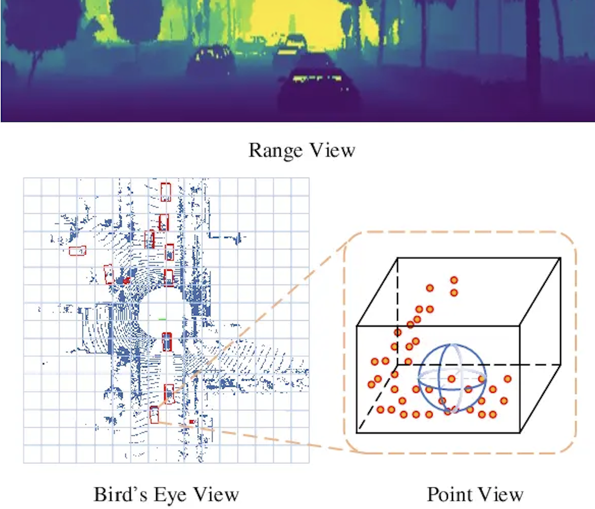
Following this previous work, they use a 2D CNN to extract features from the range view of the LiDAR. Specifically, they project the 3D points $(x,y,z)$ of the lidar onto a sphere and then convert them to image coordinates $(u,v)$ with the following equations (is this the Ball query concept I covered in PointNet?):

$$\left(\begin{array}{c}u\\ v\end{array}\right)=\left(\begin{array}{c}\frac{1}{2}\left[1-\arctan (y,x){\pi }^{-1}\right]w\\ \left[1-\left(\arcsin (z{r}^{-1})+f_{up}\right)f^{-1}\right]h\end{array}\right)$$

• $r$ represents the range of each point as $r=\sqrt{x^2+y^2+z^2}$
• desired height and width $[h,w]$
• $f=|f_{down}|+|f_{up}|$ is the sensor’s vertical FOV.

By extracting these features, they transform the problem from point-cloud moving segmentation to image moving segmentation. Here again, TNO did something interesting.

Residual Images

The residual image and range view based on LiDAR point cloud are used as the input of the segmentation network, and the temporal information in the residual image is used to distinguish the static object and the pixels on the moving object, so the actual moving object and the static object can be distinguished.

To go from a scan $k$ to a scan $l$, they save the points $p_i$ as homogenous coordinates and apply succesive transformation matrices between $N+1$ scan poses, i.e. $T_k^l\in {\mathbb{R}}^{4\times 4}$ using the following equation: $S^{k\to l}=\left\{{\prod }_{j=k}^{l+1}{T}_j^{j-1}{p}_i|p_i\in S_k\right\}$, where $S_k$ is the SLAM history $S_k=\left\{p_i\in {\mathbb{R}}^4\right\}$.

So as a summary, they first compensate the ego-motion according to the succesive transformations, and then the past scans are re-projected to the current range image view using the equation from the prior idea (going to pixel coordinates).

• To calculate the residual $d_{k,i}^l$ for each pixel $i$, they use the normalized absolute difference between the range of the current frame and the transformed frame to calculate

$$d_{k,i}^l=\frac{|r_i-r_i^{k\to l}|}{r_i}$$

• $r_i$ is the range value from $p_i$ to the current frame at the image coordinates $(ui,vi)$
• $r_i^{k\to l}$ is the range value from the transformed scan to the pixel in the same image

So in practice, the displacement of a moving car is relatively large compared to the static background, and the residual image is obvious, while the residual image of the slowly moving object is blurred and the residual pattern is not obvious. look in the reference paper and see if you find a picture to show.

• Finally, they concatenate the residual image and the range view and feed it as input to the segmentation network.

Network Architecture

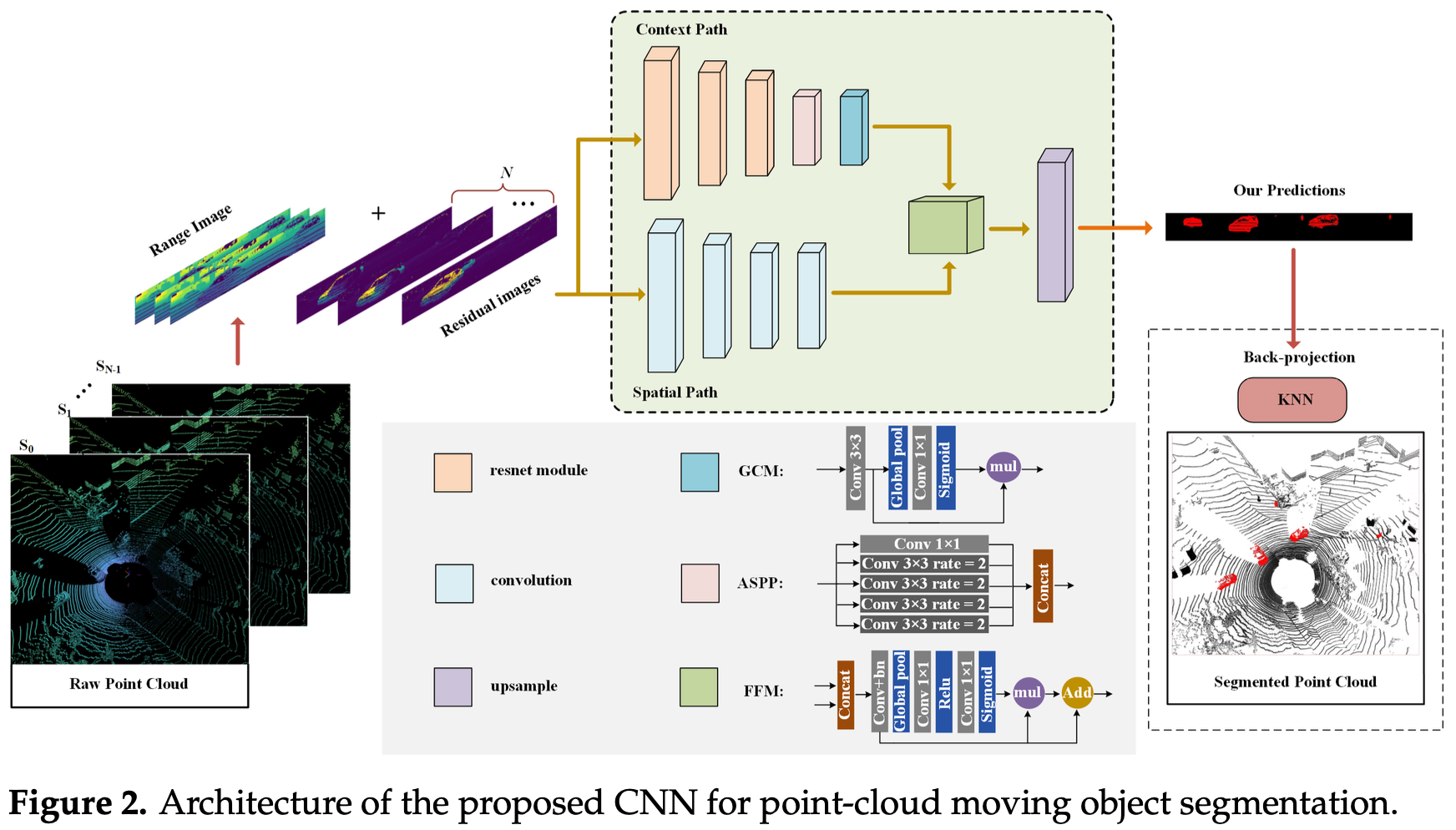
They divide it into context path and spatial path.

• The backbone of the context path is ResNet-18 to rapidly downsample the image (8x), then passes features through ASPP (which applies convolutions at multiple scales to capture objects at different sizes) and a Global Context Module (GCM, basically a global average pool + 1×1 conv) to get a broad understanding of the scene context.
• The spatial path is only four convolutional layers with $stride=2$ to preserve fine spatial detail at 1/8 resolution, keeping the high-resolution information that the context path loses during heavy downsampling. So it’s kind of making up for the down-sampling.
• The two branched are then merged in the Feature Fusion Module (FFM) using concatenation and an attention mechanism, since the two branches operate at different scales and cannot be summed.
• Instead of expensive skip-connection upsampling (e.g. UNet), they use their personal contribution - bilinear interpolation x8 to get back to the original resolution. This is the key hardware-friendly trade-off that makes it fast on FPGA.
• The two-path concept is taken from BiSeNet (2018).

Training Setup

• Framework: PyTorch, single RTX 3090Ti
• Input: 64×2048 range images + residual images, concatenated as input to the CNN
• Labels: binary masks (moving vs. static)
• Learning rate: 0.01, weight decay: 1e-4

The preprocessing consists in the first two topics covered in this section.

Dataset and Evaluation

They remaped the 28 annotated classes from SemanticKITTI into just two: moving and static. They used sequences 00-10 for training, 08 for validation, 11-21 for testing (22 in total). To evaluate the MOS performance, they use the official guidance - Jaccard index or IoU:

$$\text{IoU}=\frac{\text{TP}}{\text{TP + FP + FN}}$$

• it measures the overlap between predicted and ground truth moving pixels. A score of 1.0 means perfect, 0.0 means no overlap.

That’s really all there is to it. The only decision worth noting is their choice to collapse 28 classes into 2 — this is what makes it a binary segmentation problem rather than a full semantic one, which is why their lightweight network can handle it.

Tables 1 and 2 show an accuracy/efficiency trade-off, not a claim of superiority. Their model lands at 51.3% test IoU, below LMNet’s 62.5%, but above BiSeNet and SalsaNext - which they justify by the fact that their model uses only 34% of LMNet’s parameters and runs faster. So this is really directed towards edge computing or low-resource environments.

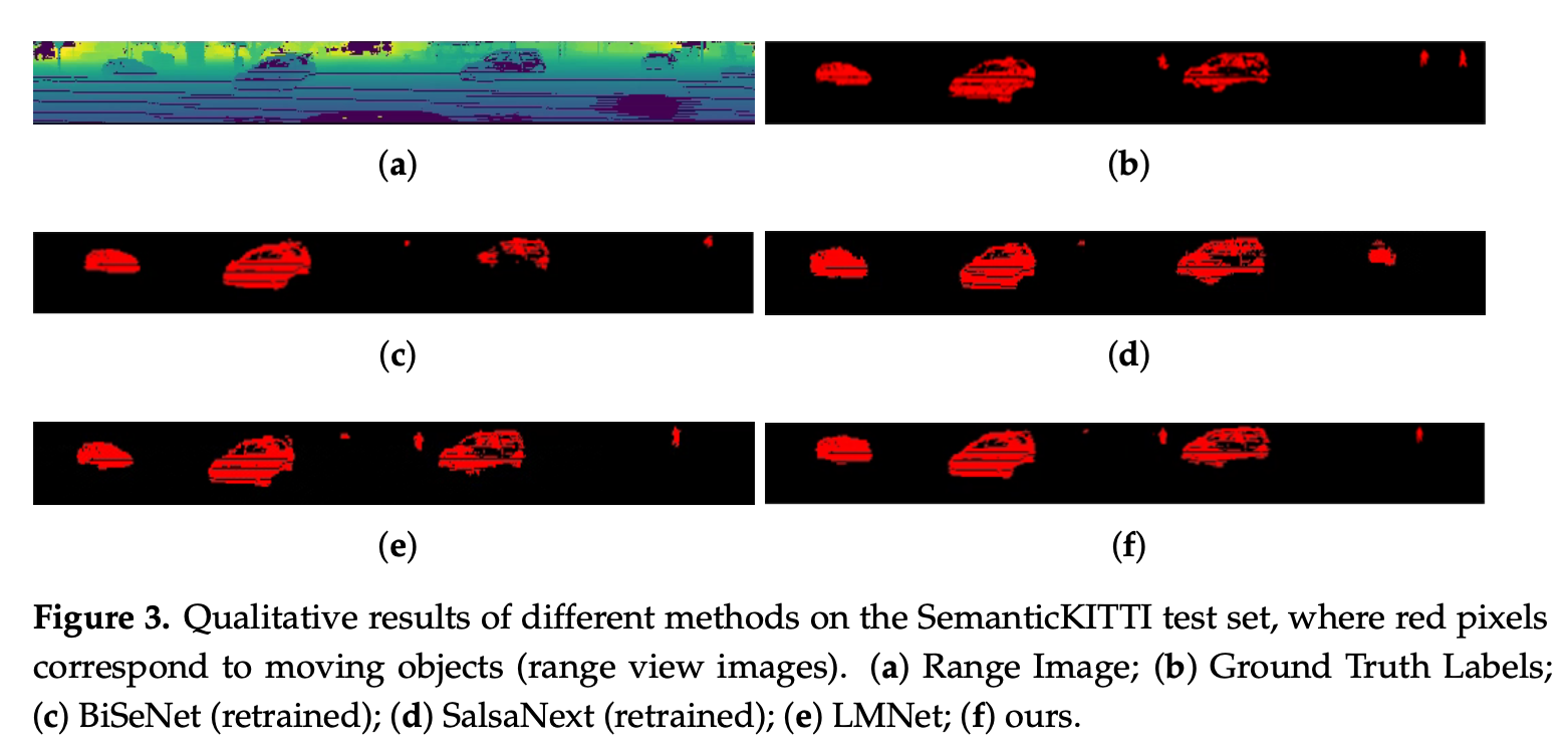
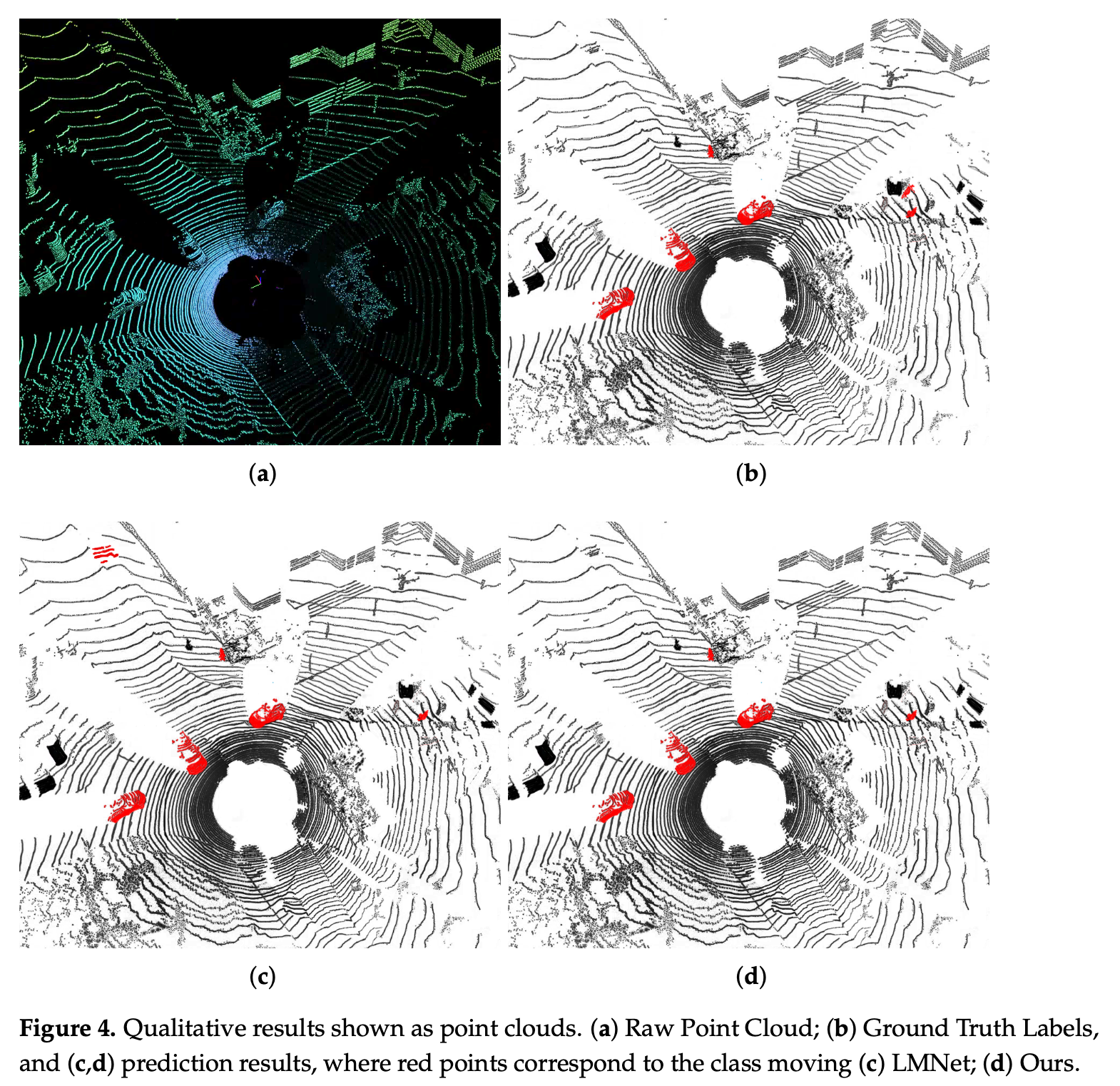
The Figures also show really close performance to LMNet, which can be called impressive, considering the size reduction and limited resources on which it can run.

Justifications

The ablation study shows they systematically added components one by one to prove each part actually contributes and earns their place.

Table 3 shows the progression:

• Context path alone: 33.6% IoU
• Adding spatial path (with simple summation): 43.2% — big jump, confirms the dual-branch idea works
• Replacing sum with FFM: 45.1% — attention-based fusion beats simple addition
• Adding GCM: 47.4%
• Adding ASPP: 52.4% — final model

Table 4 compares two post-processing methods for mapping predictions back from 2D to 3D:

• KNN (52.4%) beats CRF (Conditional Random Field) (49.1%).

The reason they give is intuitive: CRF works in 2D image space, but the problem is inherently 3D: different 3D points can project to the same 2D pixel. KNN operates in 3D space directly, so it handles boundary ambiguity better.

Run-Time Evaluation on GPU

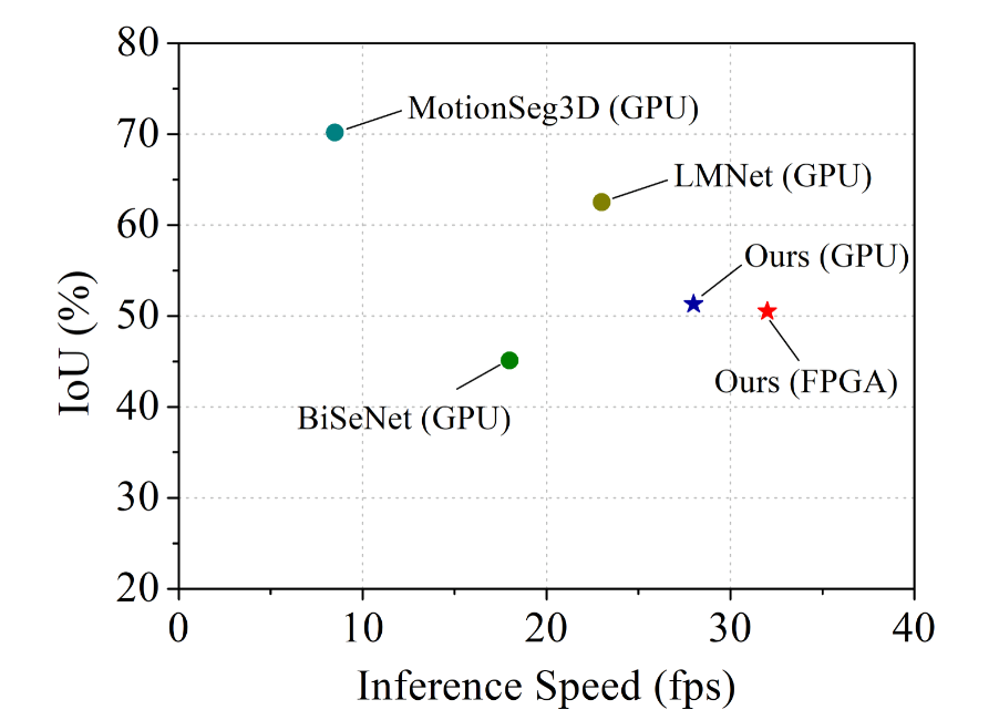
• Table 5 simply shows that they're faster, ~3x smaller, at the cost of ~11\% IoU.
• Their fps suggests that the network is never going to be the bottleneck in a real driving system.
• The Figure is exactly where an embedded autonomous driving system needs to be

Hardware Architecture

The system is split in two parts.

1. ARM core (PS side) which handles the pre/post-processing — basically everything that doesn’t need to be fast.
2. FPGA (PL side) which runs the actual NN using an NVDLA-like accelerator. Some design choices include:
   1. Finite State Machine (FSM) instead of a microcontroller to sequence CNN operations, which makes the whole process simpler and more efficient.
   2. INT8 quantization which reduces weights from 32-bit to 8-bit integers, cutting memory and compute roughly 4x.

Somehow, it ties it all together. It supports their design choices like the bilinear interpolation and it suggests the network was designed while keeping the hardware in mind.

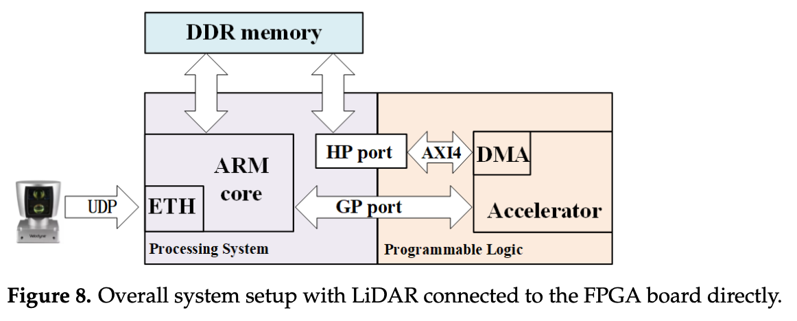
• The LiDAR is connected directly via Ethernet (UDP Protocol)
• The ARM processor receives point cloud data and stores it in DDR memory, which the NVDLA accelerator then fetches

Their results are quite stunning, with the FPGA being faster than the GPU, and doing it at 12.8W, compared to the 600-650W required by the GPU-based SalsaNext solution. There is a ~50x less power consumption on the embedded deployment. Since they mentioned they are among the first people to do the implementation on FPGA, they acknowledge that they can’t do a like-for-like hardware comparison with other work.

Also, other resources get used up to ~50%, but when it comes to the DSP (Digital Signal Processing), which is the dedicated, hard-coded hardware blocks designed to accelerate mathematical computations, they reach 91.84% (almost maxed out).

Their future improvements sound pretty vague to me. Overall decent paper with weird phrases and somewhat interesting results. However, they were expected.