Simultaneous Localization and Mapping (SLAM)

Specifically, Lidar-Inertial SLAM.

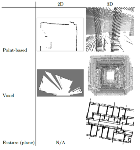
The basic idea is you build a map and then localize the robot on that map. I discussed in Lidar-Inertial Perception the types of map representations and also the scan matching methods.

GraphSLAM

“Given all sensor measurements and motion constraints collected so far… What is the most probable set of robot poses and map variables?”

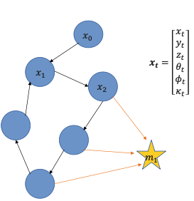
• In graph representation, all robot states are discretized into nodes
• Nodes are robot poses (circles) or observed features (stars)
• Link indicate
• transformations (𝑹, 𝒕) between consecutive poses (i.e. spatial constraints)
• observations of features, i.e., perception measurements

This means that this factor graph is a topological map.

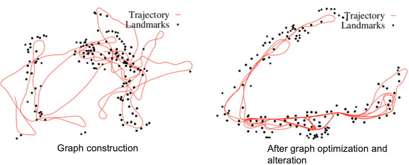
Since every edge corresponds to a spatial constraints between two nodes, we need to optimize the graph:

• Minimize the error introduced by the two constraints (alter nodes and change links)

STATE SPACE

We consider the position and orientation as the states: ${\mathbf{x}}_t\in S$

If we consider a 2D graph, then one robot state is equivalent to ${\mathbf{x}}_t=\left(\begin{array}{c}x\\ y\\ \theta \end{array}\right)$

How to discretize the trajectory so that the problem is computationally sound?

We use the key frames concept from Lidar-Inertial Perception. We discretize the trajectory w.r.t. time $\Delta t$, or by saying that there can be only one state per traveled distance (e.g. $d_0=0.1m$)

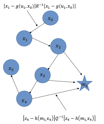
Motion Constraint

Since we are talking about Lidar-Inertial SLAM, the IMU tells us how the robot moved or the control input $u_t=\left(\begin{array}{c}{v}_t\\ {\omega }_t\end{array}\right)$.

$$\left(\begin{array}{c}{x}_t\\ y_t\\ {\theta }_t\end{array}\right)=\left(\begin{array}{c}{x}_{t-1}\\ y_{t-1}\\ {\theta }_{t-1}\end{array}\right)+\left(\begin{array}{c}\frac{-v_t}{{\omega }_t}\sin {\theta }_{t-1}+\frac{v_t}{{\omega }_t}\sin ({\theta }_{t-1}+{\omega }_t\Delta t)\\ \frac{v_t}{{\omega }_t}\cos {\theta }_{t-1}-\frac{v_t}{{\omega }_t}\cos ({\theta }_{t-1}+{\omega }_t\Delta t)\\ {\omega }_t\Delta t\end{array}\right)$$

We denote $g=g(u_t,{\mathbf{x}}_t)=\left(\begin{array}{c}{x}_{t-1}\\ y_{t-1}\\ {\theta }_{t-1}\end{array}\right)+\left(\begin{array}{c}\frac{-v_t}{{\omega }_t}\sin {\theta }_{t-1}+\frac{v_t}{{\omega }_t}\sin ({\theta }_{t-1}+{\omega }_t\Delta t)\\ \frac{v_t}{{\omega }_t}\cos {\theta }_{t-1}-\frac{v_t}{{\omega }_t}\cos ({\theta }_{t-1}+{\omega }_t\Delta t)\\ {\omega }_t\Delta t\end{array}\right)$ as the motion constraint.

To complete the update from one state to the next, we also need to take noise into consideration:

$$\left(\begin{array}{c}{x}_t\\ y_t\\ {\theta }_t\end{array}\right)=\left(\begin{array}{c}{x}_{t-1}\\ y_{t-1}\\ {\theta }_{t-1}\end{array}\right)+\left(\begin{array}{c}\frac{-v_t}{{\omega }_t}\sin {\theta }_{t-1}+\frac{v_t}{{\omega }_t}\sin ({\theta }_{t-1}+{\omega }_t\Delta t)\\ \frac{v_t}{{\omega }_t}\cos {\theta }_{t-1}-\frac{v_t}{{\omega }_t}\cos ({\theta }_{t-1}+{\omega }_t\Delta t)\\ {\omega }_t\Delta t\end{array}\right)+\left(\begin{array}{c}N(0,{\sigma }_x^2)\\ N(0,{\sigma }_y^2)\\ N(0,{\sigma }_{\theta }^2)\end{array}\right)$$

where we define $R^{-1}=\left(\begin{array}{ccc}{\sigma }_x^2& 0& 0\\ 0& {\sigma }_y^2& 0\\ 0& 0& {\sigma }_{\theta }^2\end{array}\right)$ as the Process noise covariance matrix.

Measurement Constraint

This is mainly about finding the landmarks and making use of the information from them. For this, we define a measurement model h which relies on landmarks ${\mathbf{m}}_i$ with signatures ${\mathbf{s}}_i$ and observer position ${\mathbf{x}}_t$.

Therefore, we can define the measurement ${\mathbf{z}}_t$ against the previously known landmark position of ${\mathbf{m}}_i$.

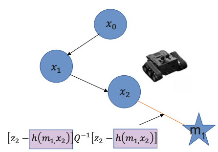
Since for this we use the Lidar, the measurement vector contains the range $r$ and the viewing angle $\varphi$ (against robot orientation $\theta$) with signature $s$:

$$z_t=\left(\begin{array}{c}{r}_t\\ {\varphi }_t\\ s_t\end{array}\right)\approx \left(\begin{array}{c}\sqrt{(m_{j,x}-x{)}^2+(m_{j,y}-y{)}^2}\\ atan2(m_{j,y}-y,m_{j,x}-x)-\theta \\ s_j\end{array}\right)+noise$$

where we define $h=\left(\begin{array}{c}\sqrt{(m_{j,x}-x{)}^2+(m_{j,y}-y{)}^2}\\ atan2(m_{j,y}-y,m_{j,x}-x)-\theta \\ s_j\end{array}\right)$ and $Q^{-1}=\left(\begin{array}{ccc}{\sigma }_r^2& 0& 0\\ 0& {\sigma }_{\varphi }^2& 0\\ 0& 0& {\sigma }_s^2\end{array}\right)$ as the Measurement noise covariance matrix.

The basic SLAM problem

These two constraints together describe a basic SLAM problem: given with the noisy control input $\mathbf{u}$ and the sensor reading $\mathbf{z}$ data, how to estimate $\mathbf{x}$ (localization) and mapping problem?

So the 4 important variables:

• ${\mathbf{x}}_t$ the pose of the robot in body frame
• $g_t$ the motion constraint using the IMU data in body frame
• ${\mathbf{h}}_t$ the measurement constraint in body frame
• ${\mathbf{z}}_t$ the measurement model which is the pose of the landmark in body frame (LiDAR)

Graph Construction

After constructing the graph, we have a cost function J to minimize. The graph contains all the measurements between time $t_0$ and $t_T$

To construct the cost function, we first define the information matrix $\Omega$ where graph links are represented in a matrix.

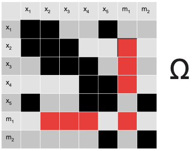
Therefore, we define:

$$J_{graphSLAM}=x_0^T{\Omega }_0{x}_0+\sum _{t=0}^T[x_t-g(u_t,x_{t-1}){]}^T{R}^{-1}[x_t-g(u_t,x_{t-1})]+\sum _{t=0}^T[z_t-h(m_{c_t},x_t){]}^T{Q}^{-1}[z_t-h(m_{c_t},x_t)]$$

Took from Section 11.4.3 of the Probabilistic Robotics book by S. Thrun:

We define $y_{0:t}$ to be a vector composed of the robot poses $x_{0:t}$ and the landmark positions $m=(m_1,m_2,\dots ,m_N{)}^T$, whereas $y_t$ is composed of the momentary pose at time $t$ and the respective landmark:

• $y_{0:t}=\left(\begin{array}{c}{x}_0\\ x_1\\ .\\ .\\ x_t\\ m\end{array}\right)$
• $y_t=\left(\begin{array}{c}{x}_t\\ m\end{array}\right)$

Linearizing the Motion Model:

The various terms in the loss function above are quadratic in the functions $g$ and $h$, not in the variables we seek to estimate (poses and the map). Thus, we have to linearize g and h via Taylor expansion around the current estimate ${\mu }_t$:

$$g(u_t,x_{t-1})\approx g(u_t,{\mu }_{t-1})+G_t(x_{t-1}-{\mu }_{t-1})$$

• Here ${\mu }_t$ is the current estimate of the state vector $y_t$.
• $G_t=\frac{\partial g(u_t,x_{t-1})}{\partial x_{t-1}}$ is the Jacobian of g at $x_t={\mu }_{t-1}$

We define the motion residual:

$$r_t^{(u)}=x_t-g(u_t,{\mu }_{t-1})$$

Then:

$$x_t-g(u_t,x_{t-1})\approx r_t^{(u)}-G_t(x_{t-1}-{\mu }_{t-1})$$

Linearizing the Measurement Model:

$$h_t(y_t,c_t)\approx h({\bar{y}}_t,c_t)+H_t(y_t-{\bar{y}}_t)$$

• ${\bar{y}}_t$ is the current estimate of state $y_t$
• $H_t$ is the Jacobian of $h$

We define the measurement residual:

$$r_t^{(z)}=z_t-h({\bar{y}}_t,c_t)$$

In class, we expand

$$H_t=\left[\begin{array}{cc}\frac{\partial h}{\partial y_t}& \frac{\partial h}{\partial c_t^i}\end{array}\right]=\left[\begin{array}{cc}{H}_t^y& H_t^{c_i}\end{array}\right]$$

The Jacobian of $r_t^z$ w.r.t. the full state vector $X$ is:

$$J_t^{(z)}=\left[\begin{array}{c}0\cdots -H_t^y\dots H_t^{c_i}\dots 0\end{array}\right]$$

• it’s a row vector (a sparse matrix row) that:
  • is zero everywhere except at the positions corresponding to:
    • the current pose $x_t$ (where we have $-H_t^y$)
    • the observed landmark $m_{ct}$ (where we have $-H_t^{c_i}$)

Example: If we are at pose $x_2$ observing landmark $m_1$:

$J_2^{(z)}=\left(\begin{array}{ccccccc}0& 0& -H_2^y& 0& \dots & -H_2^{m_1}& 0\dots \end{array}\right)$

The Full Linearization of the Cost Function:

After linearization, we substitute back into the cost function. For the measurement term:

$$\Vert z_t-h(y_t,c_t){\Vert }_{Q_t^{-1}}^2\approx \Vert r_t^{(z)}-H_t(y_t-{\bar{y}}_t){\Vert }_{Q_t^{-1}}^2$$

Let $\delta y_t=y_t-{\bar{y}}_t$ be the correction we want to find. Then:

$$\Vert r_t^{(z)}-H_t\delta y_t{\Vert }_{Q_t^{-1}}^2$$

By expanding this quadratic, we will get the contribution to $\Omega$ and $\zeta$

• Information matrix $\Omega$ (from quadratic terms $J^T{Q}^{-1}J$). It tells us which states are connected
• Information vector $\zeta$ (from linear terms $J^T{Q}^{-1}r$). It tells us how much correction is needed in each direction.

Similarly, for the motion model, we have:

$$x_t-g(u_t,x_{t-1})\approx r_t^{(u)}-G_t(x_{t-1}-{\mu }_{t-1})$$

Define the Jacobian for motion in the global state space: $J_t^{(u)}=[0\cdots -G_t\cdots I\cdots 0]$ Where: 

• $-G_t$ appears at position $i$ (for $x_{t-1}$) 
• $I$ (identity) appears at position $j$ (for $x_t$) 

The contribution to $\Omega$: 

$$\Omega \leftarrow \Omega +(J_t^{(u)}{)}^T{R}_t^{-1}{J}_t^{(u)}$$

The contribution to $\zeta$: 

$$\zeta \leftarrow \zeta +(J_t^{(u)}{)}^T{R}_t^{-1}{r}_t^{(u)}$$

Once we have $\Omega$ and $\zeta$, the solution is:

$$\Omega \delta X=\zeta$$

where $\delta X$ is the correction to apply to the current state estimate:

$$X^{new}=X^{old}+\delta X$$

Some insights:

• we can recover the covariances after solving $\Sigma ={\Omega }^{-1}$
• we iterate because linearization is only accurate near the linearization point

Now we can answer these questions:

Why isn’t integrating all odometry enough?

• Because odometry has cumulative errors (drift) that grow unbounded over time

Consider a factor graph, why is it useful to represent the robot trajectory this way?

• Sparsity (the factor graph represents only the constraints, not all correlations),
• modularity (we can add constraints incrementally)

How do nodes help with scalability when the environment gets large?

• We can discretize using the key frame concept.
• Helps with traceability.

Loop Closure

Covered in Loop Closure.

Impact on the map:

Why can a single loop-closure constraint dramatically reshape the entire map?

because Graph-SLAM solves one global least-squares problem over all poses. By directly coupling two distant poses in the trajectory, the new constraint changes the optimum for the entire problem. Consequently, many poses are adjusted simultaneously to satisfy all constraints, not just local ones

Applications for Graph-SLAM:

For example, in a forest. The tree foliage causes GNSS errors and the acquired trajectory and the point cloud is noisy. Therefore, formulating the trajectory as a graph means the poses are linked from the measured relative transformations between them. Also, the trees would appear circular and so easy to detect and insert in the Graph. Also, the method is successful only when D>>d. In this scenario, the trees are far enough apart that even with trajectory noise, the system can clearly separate observations from different trees.

Where the Method Fails:

The system breaks down in dense forests. When the distance between trees (D) becomes close to or smaller than the statistical error (d), the observations overlap.

• High Trajectory Noise: Larger drift makes the estimated position of a tree very uncertain.
• Small Feature Distance: When trees are packed together, the robot cannot distinguish if a measurement belongs to “Tree A” or “Tree B”.

Another idea: 3D Point Clouds

• Each point is a landmark
• use ICP for scan matching
• Solve for Rotation & Translation and Correct the Trajectory.

How does each sensor become just another constraint?

Sensor fusion is natural, diverse sensor data is encoded in constraints. New measurements affect only local parts of the graph, so it enables incremental and partial updates.

Data Association Uncertainty:

Often the largest and most dangerous source of error. The robot doesn’t know:

• which landmark it is observing
• which scan feature corresponds to which past feature
• whether scans overlap, or whether a loop closure is correct

Graph SLAM is in post-processing phase, so OFFLINE! It also has the largest sliding window possible: all the states ($N$).

Bayesian GraphSLAM

slides 63-70

Notes from the professor

Why is it so hard for professors to make good materials? WHHYHWQQWRQ$!@#!EWQE!@# ok

Upgrading from Pair-wise ICP to Scan-to-Map (covered in Pen and Paper Exercises SLAM):

• Instead of aligning two individual scans $(q_i\approx d_i)$, which causes drift, it’s better to scan to a local map M
• That translates into minimizing the cost function $E_m(T)={\sum }_{(p_i,m_i)}||m_i-T{p}_i|{|}^2$ where $m_i\in \text{map }M$
• This “sliding window” of recent scans provides a more stable geometric reference.

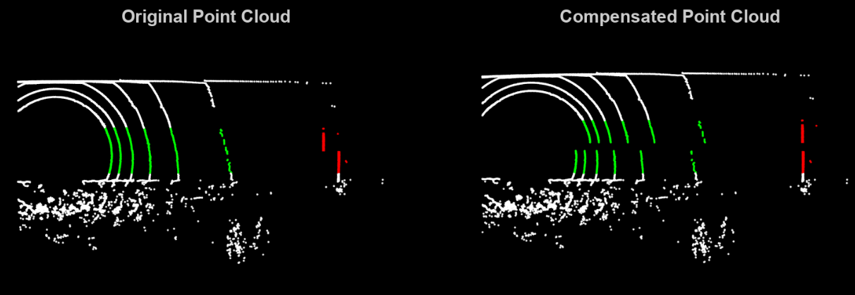
Motion Compensation (“Unwrapping”):

The notes show how we can model the motion and measurement constraints. However, when we want to implement them; we have to take into account that points were taken at different points in time $\tau \in [t_{start},t_{end}]$. If we want to align them, we need to “unwrap” them to a single reference time $t$. This actively prevents the warping of geometry (if I scan a wall, I want it to be fking straight, no?).

So the raw points $p_{raw}(\tau )$ are corrected using:

$${\tilde{p}}_{corrected}=H_{W\to B(t)}{H}_{W\to B(\tau )}^{-1}{\tilde{p}}_{raw}(\tau )$$

• The first transformation $H_{W\to B(\tau )}^{-1}$ takes the coordinates to World Frame first, and then we rearrange all of them to the Body Frame $H_{W\to B(t)}$ back again but w.r.t to time $t$.

Representing Errors in 3D (SE(3)):

We cannot subtract Rotation Matrices directly. It doesn’t really represent anything.

• So we use the Log Map to convert matrix differences into a 6D vector. It’s actually a really smart way of computing errors or optimizations.
• $r=Log(H_{meas}^{-1}{H}_{pred})\in {\mathbb{R}}^6$ yields a vector where the first 3 components are the rotation error and the last 3 errors are the translation error.

you don’t believe me? I wouldn’t! Let’s see the mathematics

We consider $H=\left[\begin{array}{cc}R& t\\ 0& 1\end{array}\right],R\in SO(3),t\in {\mathbb{R}}^3$.

The log map is $Log(H)=\left[\begin{array}{c}Log(R)\\ V^{-1}t\end{array}\right]$, where $Log(R)$ is the axis-angle vector $\varphi$ satisfying

$$R=exp(\varphi ),\theta =||\varphi ||$$

Hence, the rotation vector expresses a rotation of magnitude $\theta$ about the unit axis $u=\varphi /\theta$. The rotation logarithm is

$$Log(R)=\frac{\theta }{2\sin (\theta )}\left[\begin{array}{c}{R}_{32}-R_{23}\\ R_{13}-R_{31}\\ R_{21}-R_{12}\end{array}\right],\text{with }\theta =arccos\left(\begin{array}{c}\frac{trace(R)-1}{2}\end{array}\right)$$

I’m not gonn’ memorize all this crap. But it’s good to provide some context on how it’s actually done.

The matrix $V$ is the left Jacobian of SO(3):

$$V=I-\frac{1}{2}\hat{\varphi }+\frac{1}{{\varphi }^2}\left(\begin{array}{c}1-\frac{\theta cot(\theta /2)}{2}\end{array}\right){\hat{\theta }}^2,\hat{\varphi }=\left[\begin{array}{ccc}0& -{\varphi }_3& {\varphi }_2\\ {\varphi }_3& 0& -{\varphi }_1\\ -{\varphi }_2& {\varphi }_1& 0\end{array}\right]$$

Very similar implementation in Rodrigues Rotation Formula where I implemented using the skew symmetric logic and SO(3) space.

Redefined Global Optimization

If we take sensor fusion into consideration, we need to take all residuals into account. Thus, the trajectory is solved by minimizing a sum of residuals from different sources (IMU, LiDAR, Loop Closures). It helps since it’s how sensor fusion actually happens—by weighting each sensor based on its uncertainty. How we get here is covered in Pen and Paper Exercises SLAM.

$$\hat{X}=argmi{n}_X\left(\begin{array}{c}||r_0|{|}_{{\sum }_0}^2+\sum ||r^{IMU}|{|}_{{\sum }_{IMU}}^2+\sum ||r^{LIO}|{|}_{{\sum }_{LIO}}^2+\sum ||r^{LC}|{|}_{{\sum }_{LC}}^2\end{array}\right)$$

Each residual $r$ is weighted by its covariance $\sum$, allowing the system to trust the IMU during fast motion and LiDAR when the geometry is clear. I read somewhere that the covariance is uncertainty, so its inverse is information.

• $||r|{|}_{\sum }^2=r^T{\sum }^{-1}r$
• So intuition tells us that if uncertainty is high, the information is low. This mathematically forces the optimizer to give that measurement less “vote” in the final trajectory.