Lidar-Inertial Perception

LiDAR = light detection and ranging

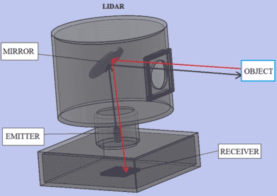
Lidars have an emitter to send light and a receiver to detect the backscattered signal. They are different to cameras in terms that a camera only has a receiver. One receiver is like a single pixel.

There different types of lidars:

• continuous-wave lidars
• pulsed lidars
• single-photon lidars

Continuous-wave lidars:

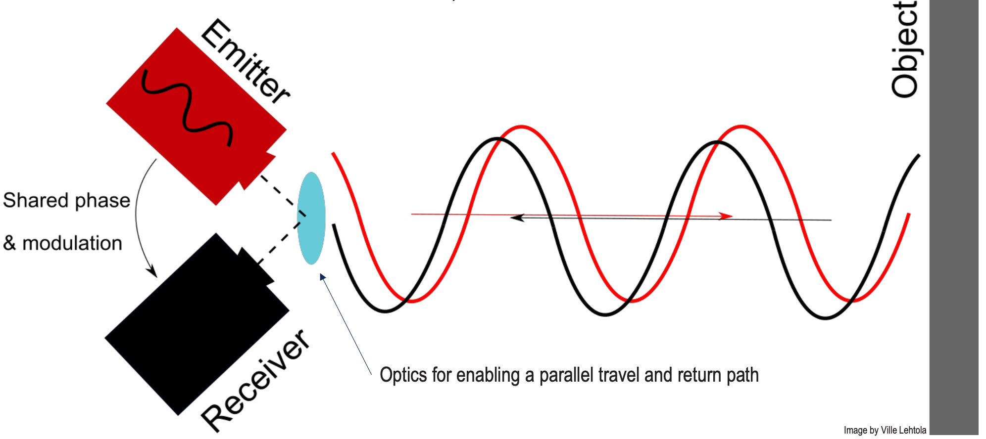
CW Lidar emits a steady light beam, unlike pulsed lidar. They work based on FMCW (Frequency Modulated Continuous Wave) which modulate the light’s frequency or phase to measure distance and velocity with high precision.

Single Photon Lidars:

• Illuminate the scene with a specific wavelength (typically 800 nm)
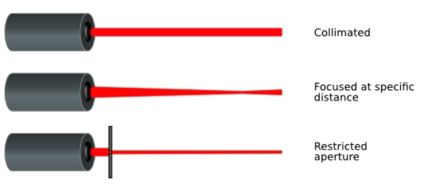
• Light can be non-collimated
• Receivers can form an array
  • Typically Single-Photon-Avalance-Diodes (SPAD)
  • Triggered when the first photon within a narrow bandwidth arrives
• Limitations: very susceptible to background illumination (=direct and diffuse sunlight)

Pulsed Lidars:

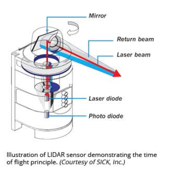
TIME-OF-FLIGHT (TOF) MEASUREMENT is done to obtain the range to the object. A collimated light pulse is emitted, travels to the object, and then is backscattered to the receiver (elementary physics type of shi)

$$r=c\frac{△t}{2}$$

where

• r is the range to the target
• c is the speed of light
• $△t$ is the time between pulse emission and reception
• Factor of 2, because the pulse flies back and forth

The Design:

• Typically, lidars require energy (more than cameras) because the scene needs to be illuminated for measurements.
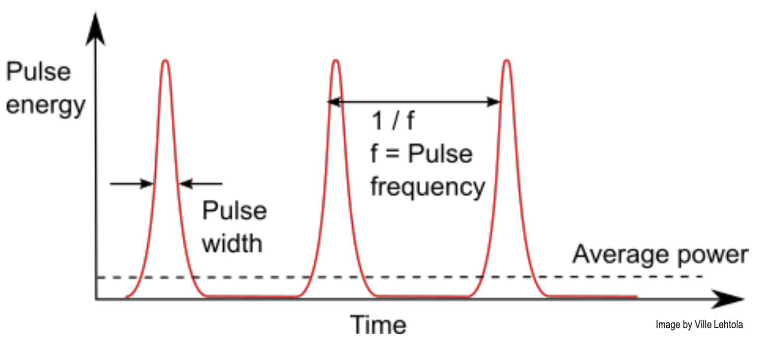
• Pulse energy needs to be high if a long range is needed
• Having collimated beams avoids the energy from being dispersed
• Pulse frequency is important to get a sufficiently high point cloud density (”point resolution”)

Most important properties include Frequency, Resolution, Accuracy, Precision (applies to all types of sensors).

Coordinate Frame for 2D LiDAR

Polar Coordinates

We have two vectors which define the polar coordinates, vector $\hat{r}$ which changes the radius of the compass and vector $\hat{\theta }$ which changes the angle $\theta$. $\hat{\theta }$ is perpendicular to $\hat{r}$ (and is thus, orthogonal). $\hat{\theta }$ is called the azimuthal vector.

$$p_{polar}^s=(r,\theta )$$

where

• $r\in [min\_range,max\_range]$
• $\theta \in [0,360]$

Cylindrical coordinates

are basically polar coordinates in 3D. We follow the left hand rule and thus $r$ is the first vector, $\theta$ is the second vector and $z$ is the third vector.

Conversion from Cartesian to Polar Coordinates

We simply let

• $x=r\cos \theta$
• $y=r\sin \theta$

And define $p_{xyz}^s=(x,y,z=0{)}^T$

To get a point in body frame, we do:

$$p^b=R_s^b{p}^s+t_s^b$$

To get a point in the ECEF frame, we need to use IMU+GNSS for orientation:

$$p^e=R_b^e(R_s^b{p}^s+t_s^b)+t_b^e$$

Questions

What is needed to measure far away?

• It’s basically a design choice. Since more power requires more energy, it’s basically a cost decision?

What does a pulsed lidar measure?

• It measures the range to the target using the time-of-flight measurement equation from physics.

Which lidar type does amplitude, frequency, or time modulation?

• The frequency modulated continuous wave lidars (fmcw lidars) use frequency modulations.
• Pulsed lidars and single-photon lidars use time modulation

3D LiDARS

They basically give us the 3D point cloud in body frame.

MAP Representations

This is how a robot can understand the world. A map can be represented through:

• Metric Maps
  • Point Clouds
  • Voxels (or rasters)
  • Features (or vectors)
  • Meshes
• Topological Maps
  • Factor graph: a pose graph and a landmark graph
  • Semantic graphs / Scene graphs
• Hybrid Maps
  • Semantic and metric information together

Metric Maps

They are point-based maps. In 2D, they are represented through occupancy grids.

Topological Maps

They represent the environment as a graph where:

• Nodes: Locations, places, regions
• Edges: Connectivity between nodes, such as traversable paths

Semantic Graphs: Focus on objects and their relationships within a scene

• Nodes contain semantic labels (e.g., “chair,” “door”)
• Edges describe spatial relationships (e.g., “next to,” “on top of”).

Scan Matching

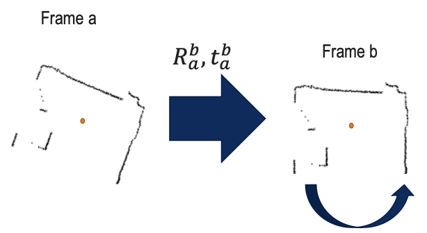
• Check difference between two latest frames a and b
• Calculate translation and rotation using ICP (Iterative Closest Point)
• Run algorithm with a high frequency to keep up with the motion
• Keeps translations and rotations small!

Iterative Closest Point (ICP) Algorithm

Goal: Estimate the transformation to move one cloud so that it is aligned with the other.

Detailed more at ICP.

Problem in Scan Matching: Lidar errors may cause drift. Looking at two very similar scans gives a lot of weight to the noise — especially when the robot is stationary since there should be no drift.

Solution:

• Use a keyframe (first introduced in PTAM)
  • Store one scan as a keyframe
  • Check updates against the keyframe, not against the previous frame. This way, we don’t process every single new frame that don’t add information.
  • Update the keyframe when the sensor moves significantly, e.g., 10 cm or 0.1 degrees

More tricks include noise handling through markers or features, or use an IMU for the theta prediction of the scan registration.

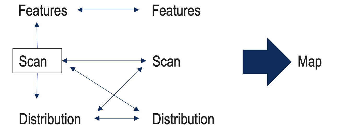
Matching Techniques

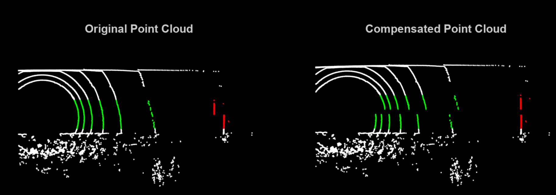
Lidar-Inertial Fusion

Context: a spinning lidar collects points sequentially over time, leading to motion distortions if the sensor moves or rotates during data acquisition. This results in points in the point cloud don’t accurately represent their real-world positions because the lidar’s frame of reference changes during the scan.

Solution: IMU preintegration is a process that uses high-frequency inertial measurements (linear accelerations and angular velocities) to estimate the sensor’s pose (position and orientation) changes over time.

Rotation is the most critical to minimize in ICP formalism.

• IMU saves multiple ICP iterations
• CPU effort saved

ICP SLAM

We need to take uncertainty into account with Gaussian Distributions. In addition to the pose X, the pose estimate $\bar{\mathbf{X}}$ and the pose error $\Delta \mathbf{X}$ are required.

The positional error of a scan at its pose X is described by:

$$E=\sum _{i=1}^m\Vert \mathbf{X}\oplus {\mathbf{d}}_i-{\mathbf{m}}_i{\Vert }^2=\sum _{i=1}^m\Vert {\mathbf{Z}}_i(\mathbf{X}){\Vert }^2$$

Here, $\oplus$ is a compounding operation that transforms a point ${\mathbf{d}}_i$ into the global coordinate system. For small pose errors $△X$, E can be linearized through Taylor Series Expansion:

$${\mathbf{Z}}_i(\mathbf{X})\approx \bar{\mathbf{X}}\oplus {\mathbf{d}}_i-{\mathbf{m}}_i-\nabla {\mathbf{Z}}_i(\bar{\mathbf{X}})\Delta \mathbf{X}$$ $${\mathbf{Z}}_i(\mathbf{X})={\mathbf{Z}}_i(\bar{\mathbf{X}})-\nabla {\mathbf{Z}}_i(\bar{\mathbf{X}})\Delta \mathbf{X}$$

Utilizing the matrix decomposition $M_{i}H$ of $\nabla {\mathbf{Z}}_i(\bar{\mathbf{X}})$ (i.e. the Jacobian) that separates the pose information $\mathbf{X}$, which is contained in $\mathbf{H}$, from the points information ${\mathbf{m}}_i$ and ${\mathbf{d}}_i$, which are contained in ${\mathbf{M}}_i$

$${\mathbf{Z}}_i(\mathbf{X})\approx {\mathbf{Z}}_i(\bar{\mathbf{X}})-{\mathbf{M}}_i\mathbf{H}\Delta \mathbf{X}$$

Because ${\mathbf{M}}_i$ is independent of the pose, the positional error E is approximated as

$$E\approx (\mathbf{Z}-\mathbf{MH}\Delta \mathbf{X}{)}^T(\mathbf{Z}-\mathbf{MH}\Delta \mathbf{X})$$

where $\mathbf{Z}$ is the concatenation of all ${\mathbf{Z}}_i(\bar{\mathbf{X}})$ and $\mathbf{M}$ the concatenation of all ${\mathbf{M}}_i$‘s

E is minimized by the ideal pose

$$\bar{\mathbf{E}}=({\mathbf{M}}^T\mathbf{M}{)}^{-1}{\mathbf{M}}^T\mathbf{Z}$$

and its covariance is given by

$$\mathbf{C}=s^2({\mathbf{M}}^T\mathbf{M})$$

where $s^2$ is the unbiased estimate of the covariance of the identically, independently distributed errors of ${\mathbf{Z}}_i$

$$s^2=(\mathbf{Z}-\mathbf{M}\bar{\mathbf{E}}{)}^T(\mathbf{Z}-\mathbf{M}\bar{\mathbf{E}})/(2m-3)$$

Note that $\bar{\mathbf{E}}$ is the minimum for the linearized pose $\mathbf{H}\Delta \mathbf{X}$. To obtain the optimal $\mathbf{X}$ the following transformation is performed:

$$\mathbf{X}=\bar{\mathbf{X}}-{\mathbf{H}}^{-1}\bar{\mathbf{E}}$$ $$\mathbf{C}=({\mathbf{H}}^{-1})\mathbf{C}({\mathbf{H}}^{-1}{)}^T$$

The representation of pose $\mathbf{X}$ in Euler angles, as well as its estimate and error is as follows:

$$\mathbf{X}=\left(\begin{array}{c}{t}_x\\ t_y\\ t_z\\ {\theta }_x\\ {\theta }_y\\ {\theta }_z\end{array}\right),\bar{\mathbf{X}}=\left(\begin{array}{c}{\bar{t}}_x\\ {\bar{t}}_y\\ {\bar{t}}_z\\ {\bar{\theta }}_x\\ {\bar{\theta }}_y\\ {\bar{\theta }}_z\end{array}\right),\Delta \mathbf{X}=\left(\begin{array}{c}\Delta t_x\\ \Delta t_y\\ \Delta t_z\\ \Delta {\theta }_x\\ \Delta {\theta }_y\\ \Delta {\theta }_z\end{array}\right)$$