Error Analysis of Airborne Laser Scanning Data

This lecture was divided in two parts — Error Analysis (1) and Strip Adjustment (2).

Error Analysis

Laser scanners consist of three different sensors. A lot of issues can go wrong with the individual sensors as well as with their integration. Sources of error in ALS data fall into systematic height errors (strip-to-strip height offsets), planimetric offsets (from INS alignment, GPS, calibration errors), and scanner artefacts (e.g. polygon mirror miscalibration causing odd/even scan line differences).

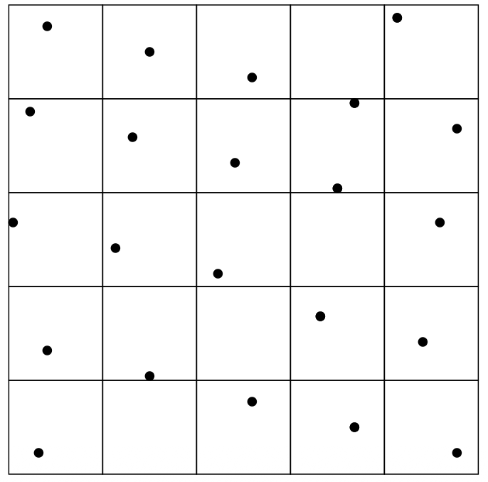
Imaging point clouds: use binning to define a raster and for each raster cell I can see if I have points inside. If there is, I assign a height to each point in that cell.

Though this may leave empty bins.

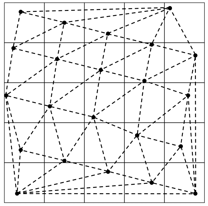
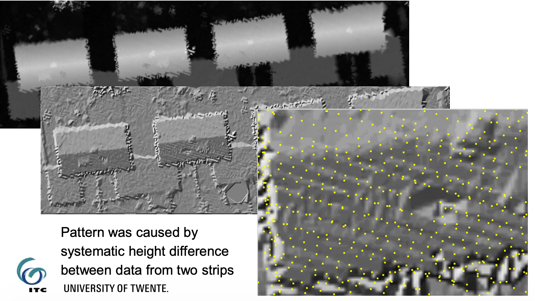
I can use interpolation techniqueslike Nearest neighbor, TIN, Splines. In the Figure, he used triangulation (TIN).

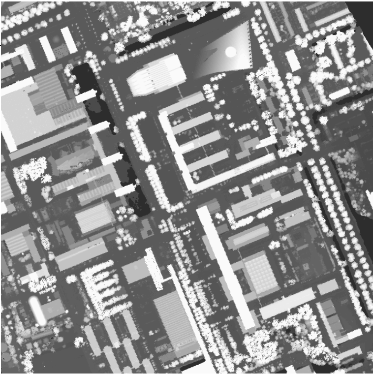
Quantisation is converting heights to grey value range 0-255. There you get a histogram and the low points are the ground. You get a lil bit of over saturation, but you need to move 255 a lil bit to the left to not get over-darkened images.

Why is it even mentioned? if you naively map the full range linearly, subtle height differences in flat areas (like a terrain with small bumps) might all collapse into the same grey value and become invisible. So the mapping needs to be chosen carefully based on what you want to see. The histogram also helps you understand which regions are more prominent than others and which might benefit from extra attention.

Pseudo Shading

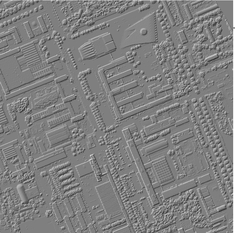
It is the next step that follows quantisation. For this, we use Roberts gradient $k=\left(\begin{array}{cc}-1& 0\\ 0& 1\end{array}\right)$, $g^{\prime }=k\ast g$ to the grey value image to make terrain pop visually. I can go into second and third derivatives. Use $\log$ to handle big values? They are not derivatives, they are simply steps.

• $g^{\prime }$ is the gradient of the image
• $g^{\prime \prime }$ compresses large gradients
• $g^{\prime \prime \prime }$ rescales to 0-255 range.

Left image is Quantisation and right image is after applying Pseudo Shading.

Data Completness

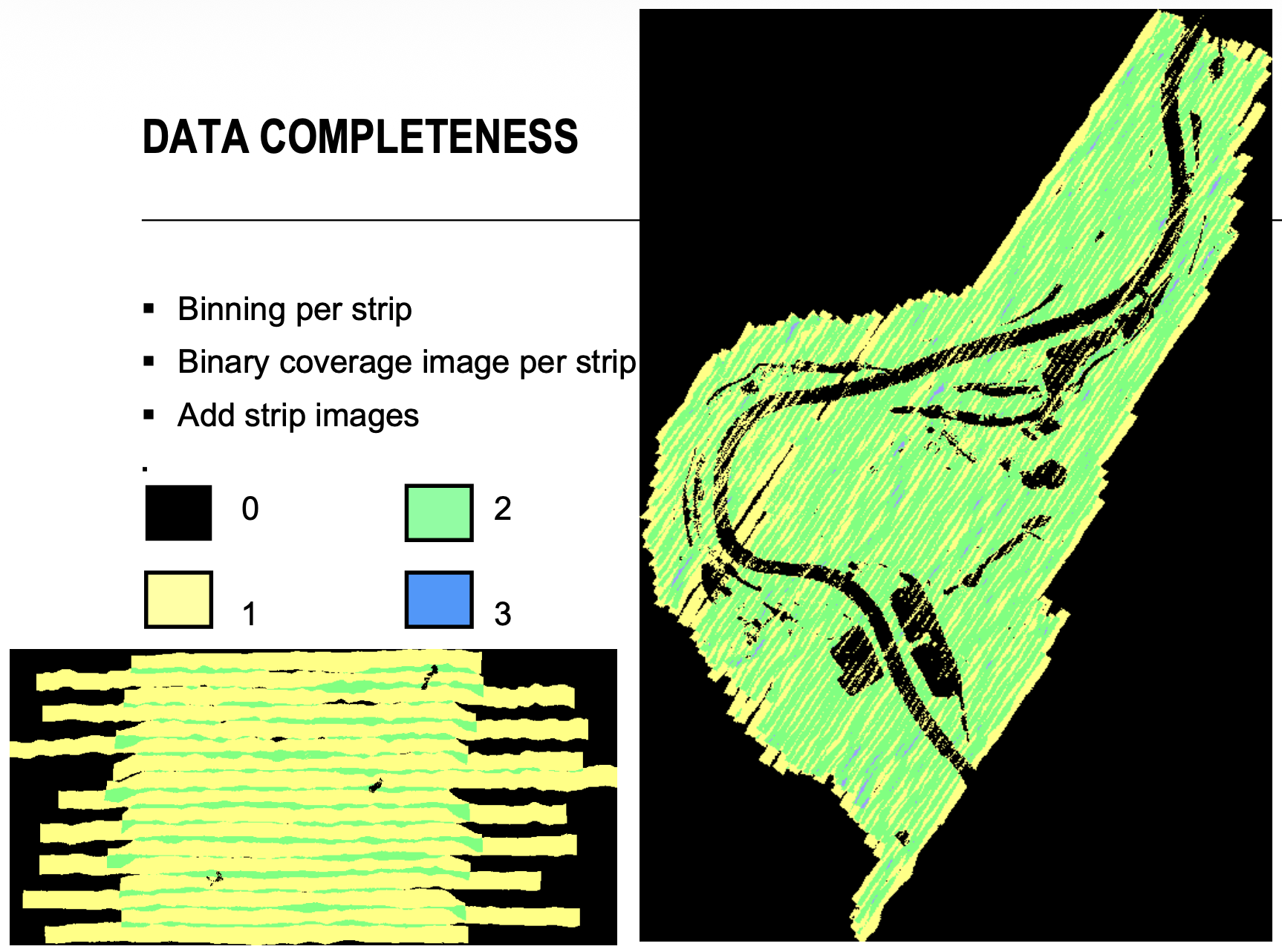
We need to ask “Has all the data been collected? Is it complete?”.

• Binning per strip: they just use a binary mask. 1 - there is data in a raster cell, 0 - there is not. You add up and get the image on the right. The color indicates in how many flight lines the data has been collected. What you don’t want is the empty spaces. Here you can check if you are missing any data.

It’s more advantageous to do your data collection at night. Don’t have missing parts! Your contract will be declined!

Systematic Height Errors

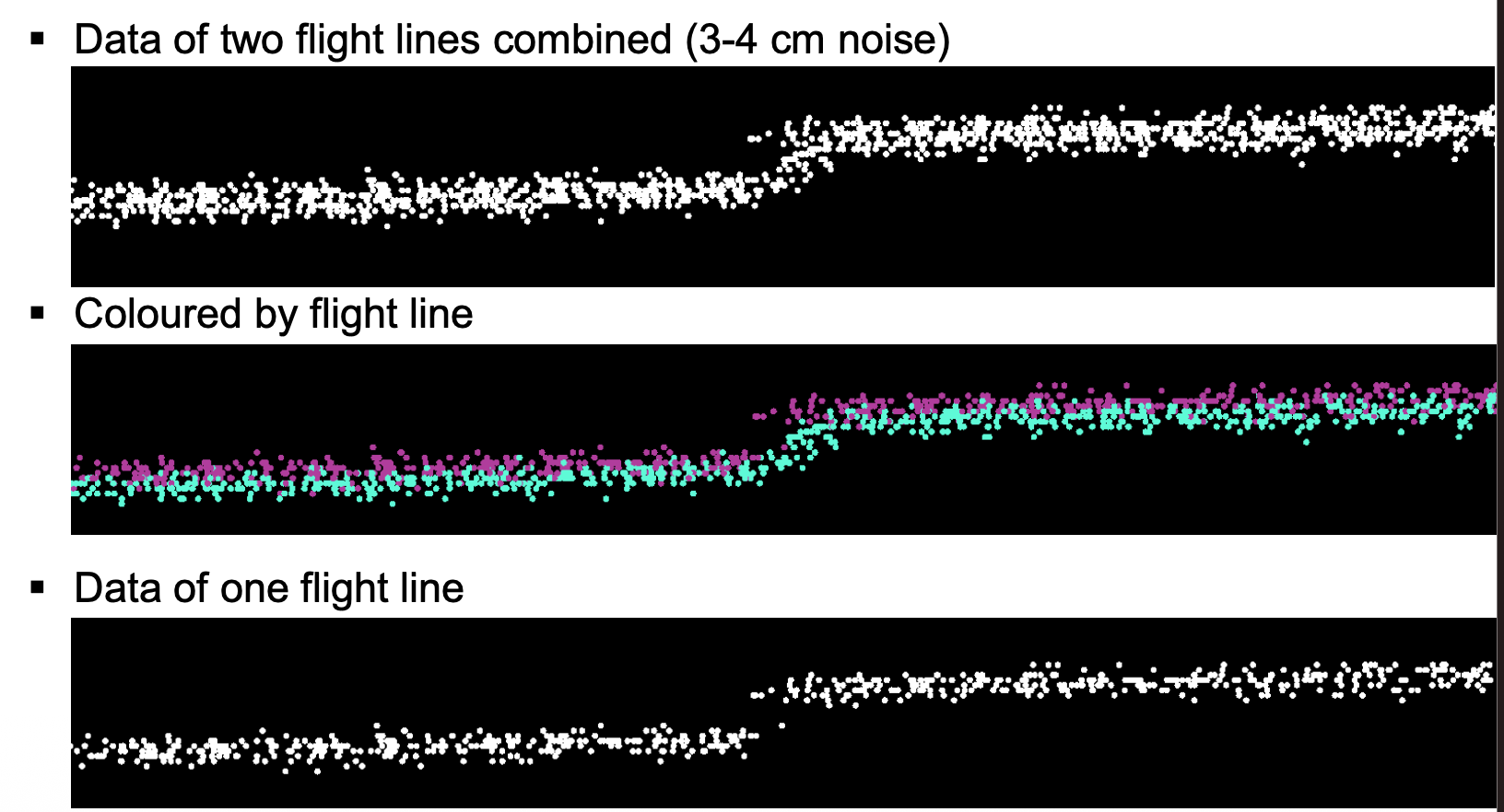
The second picture is the gradients. The cause of the weird endings of the roofs: between 2 flight lines, the height was different. The triangulation (mesh) will simply connect those points and that’s exactly what’s causing that effect.

Height offsets between strips

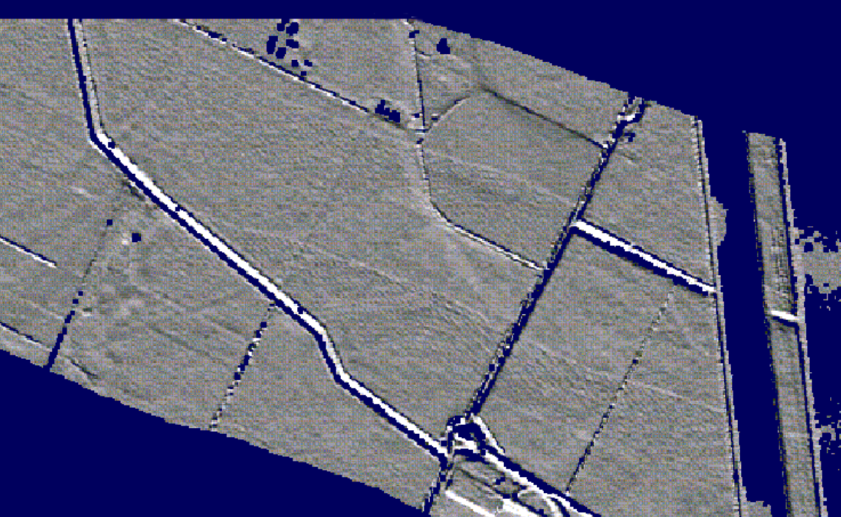
• The terrain might look bumpier in the middle region. That's because of the same reason above.

Overlaid Flight Lines

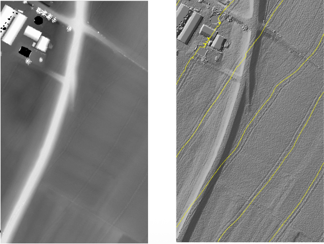
• 2-3 degrees difference in perspective give those lines.

Measurements in strip overlays

If you fly over the same area twice, you assume the area hasn’t changed in the meantime. The roofs and the ground should be pretty much the same. So if you measure the height differences, you can get nice measurements to analyze the quality of your data. You’re hoping for the mean around 0.

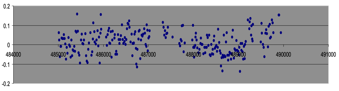
In the next slide, I see the mean is ~0.05. If I zoom in, I find the systematic patterns in the height. Those are coming from the GNSS, apparently. The IMU interpolates between those points. It’s basically the interpolation between the GNSS points.

The differences between scan lines showcased (first - the rotating mirror) and second the polygonal mirrors? It just shows bad calibration

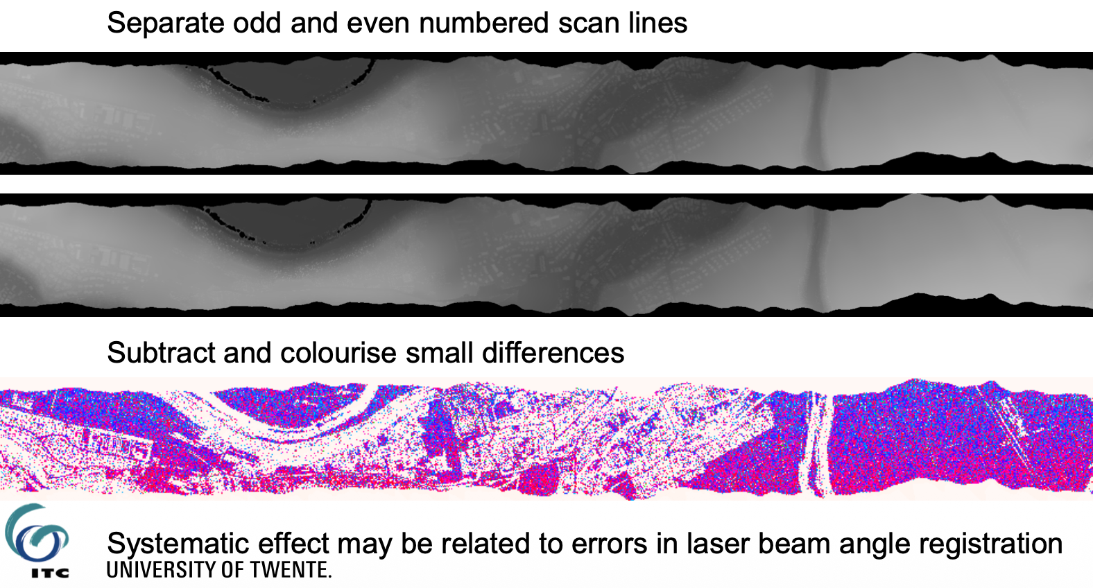
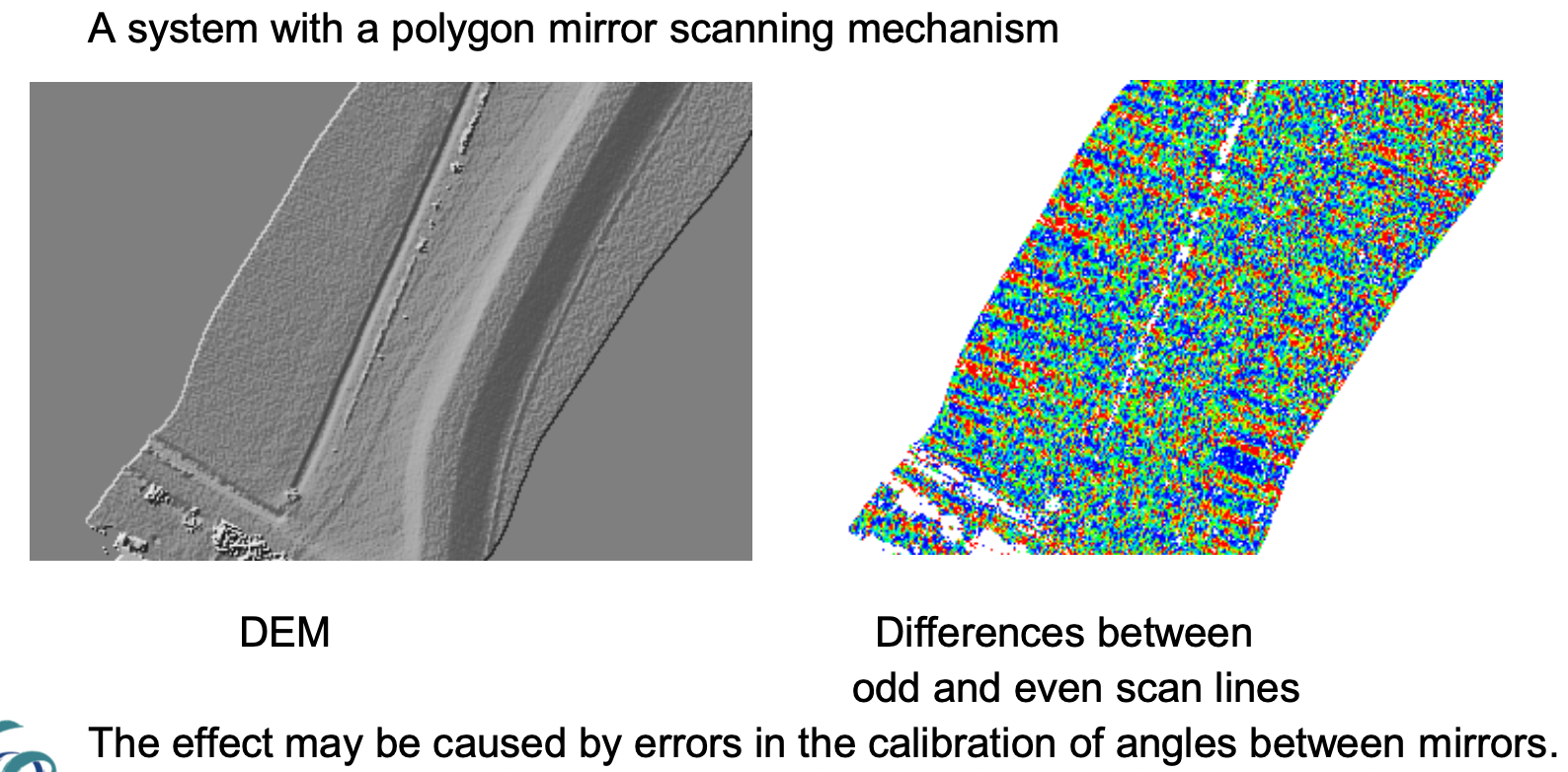
Planimetric Offsets between strips

Basically a combination of multiple errors. For example, the rotation between the IMU and Laser scanner itself. In the figure below, the errors accumulate and we can see how the data of two different flight lines are shifted

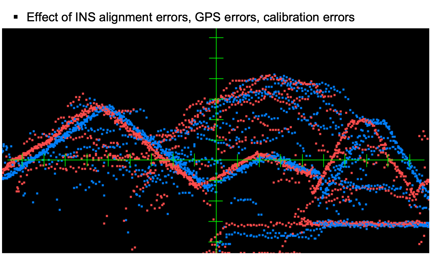
• basically calibration errors. Planimetric errors do not become visible unless you have sloped surfaces (e.g. roofs). Reflection data can also be used to align two different flight lines (take a road for example, maybe you can apply the tie points concept).

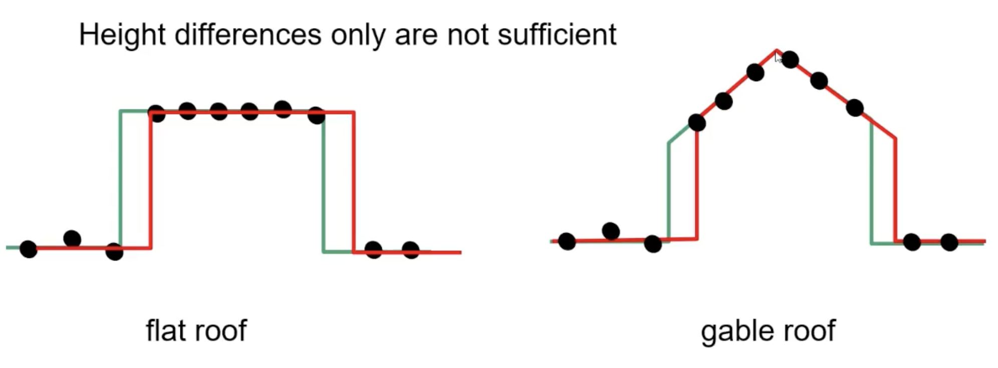
Only height is not enough to get the offset between flight lines. More features on the roofs help on this. The red lines are one flight and the green lines are the second flight. The idea is that the points can very well represent both representations. However, in the gable roof we can see the ridge lines that overlap regardless of how we see it. If you have this data, you can just shift the point cloud (mostly by using the gable roofs and adjusting for the offset in the ridge line.

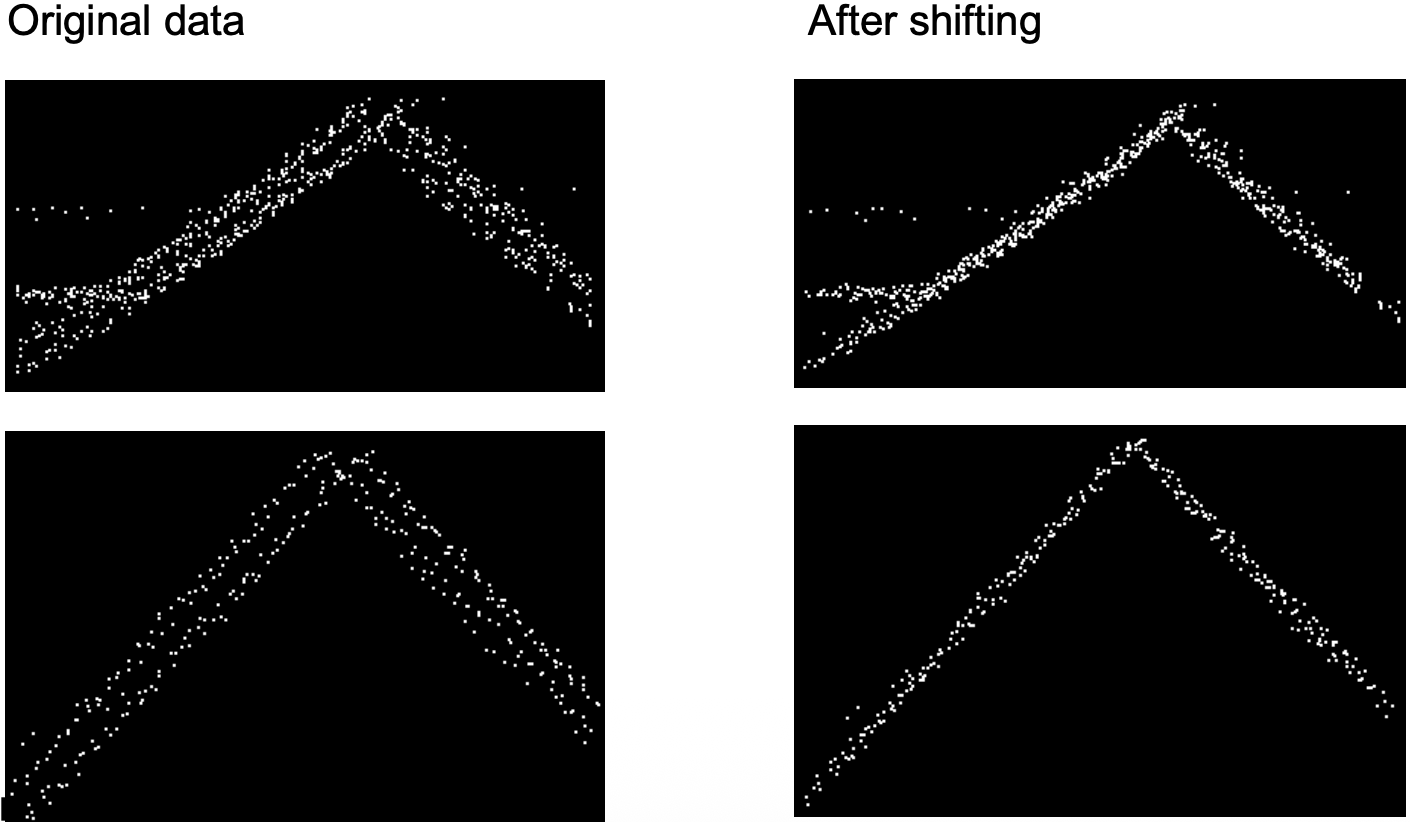
How to assess the planimetric accuracy?

• measuring distance between ridge lines in strip overlaps
• point spacing

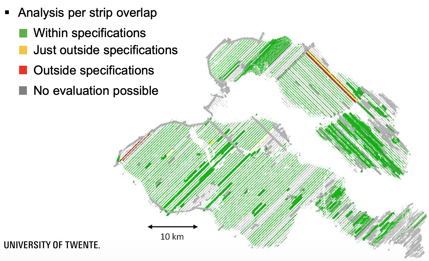
Those very thick lines usually represent that the experiment was redone on that section, therefore the high reliability.

---

Strip Adjustment of Airborne Laser Scanning Data

This is where we talk about how we solve these errors

First, ask myself if it’s really necessary.

• 0.2-0.3m for USGS DEMs
• 0.1m for more detailed DEMs
• 0.02m for water level decisions

Strip Adjustment

Aligning the multiple laser scans.

Identify the patches where you find corresponding points. That’s how we get rotation and translation from different flights.

$Z_{ref}$ could be the gps ground truth height of a point and $Z_s$ could be the point from the laser scan. Only if you have reference.

Smiley error: you have a flat terrain, but the reconstructed point cloud looks like a smiley. So if I have 3 flight lines that connect with each other, we can rotate the point clouds and apply an offset such as to minimize the distortions (you can see in the “after adjustment”). But you still have an extremely curved trend. To avoid it, we can use more reference points (can force the difference in height between strips). Another solution is to take cross strips (perpendicular). So if I assume I’m rotatin between $[-30,30]$ degrees, maybe I’m actually rotating between $[-31,31]$ degrees.

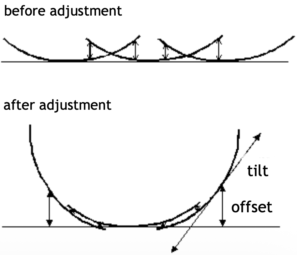
The idea is that even with minimization of errors, we still get a big error in the end (The point cloud was assumed on a flat terrain in the Figure, so it’s reeeaaaaaalllyyyy curved). Therefore, it’s still the calibration errors that should be addressed first. What was one in those strips was that they rotated the point clouds of each strip to align with each other.

1D adjustment corrects only height using offset + tilt per strip (3 parameters: $a_s,b_s,c_s$)

3-D Adjustment

I explain the differences around the center of the strip + translation. And then try to find the rotations. So in total there are 6 offset parameters in 3D (Translation + Rotation). If we consider drift that constantly changes along time, then we have 12 (6 offsets, 6 drifts). There can be 13 if we take the error in the rotating mirror as well.

Companies mostly care about improvement in height, not X and Y.

In case of slopes, the error in the viewing direction of the laser beam will have different effect on the point cloud. This can be used to estimate the angle error. In a flat terrain, we should see pretty much the same height regardless of the viewing direction. You can’t really do too much with that. Estimability matters: flat terrain only constrains height offset and roll; pitch needs slopes in flight direction; heading needs slopes in multiple directions — cross strips help significantly.

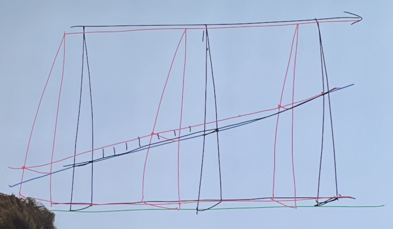
Look at the data of a single flight line and extract your features there. And then you can combined the independent data, viewed together. It’s usually simpler than trying to fix multiple things at once.