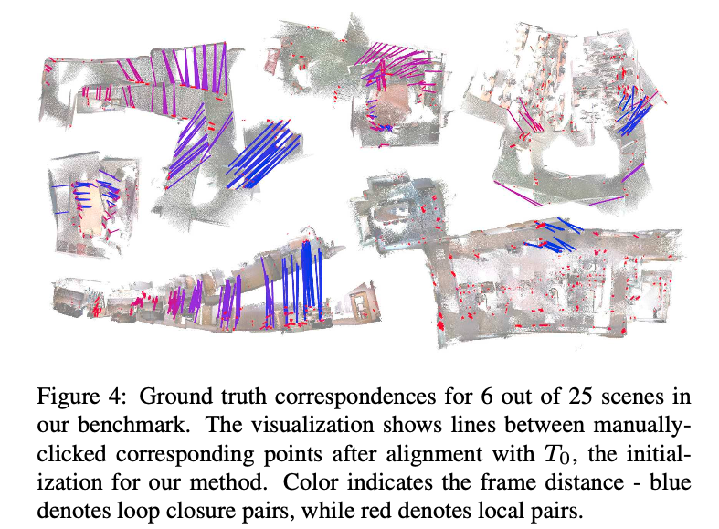
From 2017. This paper aims at RGB-D scanning of indoor environments.
Summary of the method
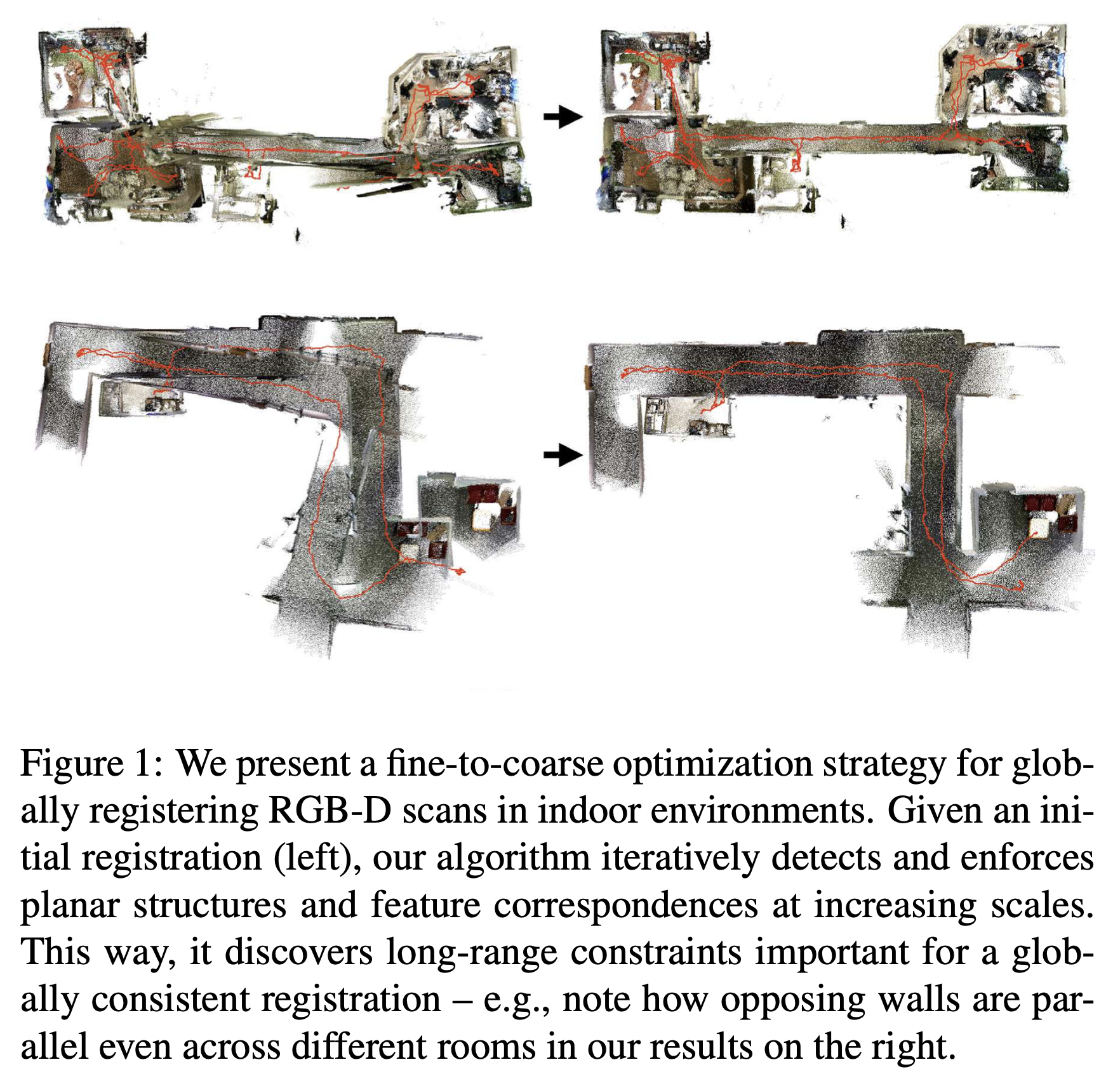
It’s a global registration algorithm that refines an initial set of camera poses by iteratively detecting and enforcing geometric constraints within gradually growing subsets of the trajectory.
In other words, registering long RGB-D sequences (hand-held camera, frames, multi-rooms) into one globally consistent 3D model. Standard pipelines (frame-to-frame tracking + loop closure) drifts and fails on large scenes, producing warped/overlapping rooms.
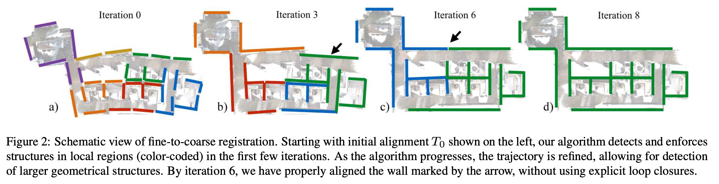
During each iteration, closest point and geometric constraints (parallelism, perpendicularity, etc.) are detected and enforced only within “windows” of neighboring RGB-D frames. The windows start small and increase in time (doubles every iteration).
- it enables detection of longer-range correspondences and large-scale geometric structures, leveraging the improved trajectory provided by previous iterations.
- continues until a single window includes the entire scan and a global refinement can be done robustly
Intuition
you can’t detect a long-range constraint (e.g. far-apart parallel walls) correctly until the geometry leading up to it is already roughly right. The growing window lets the correctness propagate.
Would VPR be a good application for detecting the loop closures in this case, I wonder
Xiao et al.’s SUN3DSfM apparently did this already. Give them a read. Also global BA.
The paper explicitly notes it fails on their corridor sequence due to repetitive/self-similar geometry — which is the key risk to be aware of.
I see they do not initialize the algorithm in any way. They simply rely on the E-M strategy to provide good results. Actually, in the preprocessing step it explains what they do — but it’s pretty much what I said.
- E-step: detecting a set of viable constraints
- M-step: continuously solving for the camera poses that best satisfy the constraints
They assume planar structure relationships (parallelism, orthogonality) it won't work on round walls.
Pretty standard in the NL for example. They use old buildings which have rounds walls and so this method simply cannot be applied on those cases.
GlobFit (Li et al.) fits and relates multiple primitive types (planes, cylinders, spheres) rather than assuming everything is a plane.
They do feature correspondence between the closest compatible features (like in ICP).
Algorithm
- Let be a RGB-D image from a set of images
- Let represent the position and orientation of the camera for
- Let be the features from all images in
- Let be the base planar regions from all images in
- Let be the coplanar base planar regions for a iteration
- Let be the set of local, pairwise alignment transformations
- Let be the feature correspondence constraints for a iteration
- Let be the structural model constraints for a iteration
- Let and be the geometrical constraints
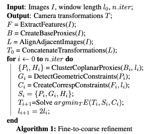
Extract and . Then estimate and concatenate these local transformations to form an initial guess for global transformations . In each iteration , they refine by first detecting both and based on detected clusters of and and between them. Then optimize the global transformations for the next iteration by minimizing an error function encoding penalties for the detected constraints. Then finish by doubling the size of the window for next iteration, .
Preprocessing
For feature detection they found planar patches and linear edges along creases and contours in depth images to be more robust.
- per pixel, every frame
Once is created, define a feature from image at iteration as where , and respectively denote the feature’s position, normal (for planar patches) and direction (for linear edges) in the camera space.
To create , they used aglomerative hierarchical clustering, where clusters of nearly co-planar features are repeatedly merged based on the compatibilities of their positions and normals. Once is created, define a proxy from image at iteration as where is the centroid of inlier features, and is the fitted normal.
To estimate , the goal is to create local alignment transformations that can be used later in the optimization to preserve the local shape of the estimated camera trajectory. Apparently they detect SIFT features in consecutive images, prune out ones without valid (missing or high) depth values, and then use RANSAC on backprojected SIFT keypoints to search for the rigid transformations aligning as many of these keypoints as possible.
- Then, the initial camera-to-world transformations is extracted by simply concatenating the estimated local transformations .
- These are locally accurate, not globally consistent.
Fine-to-Coarse Refinement
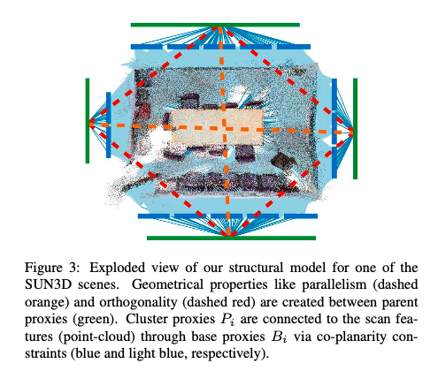
They model the co-planarity constraints by clustering the transformed base proxies into representative cluster proxies .
- this is the actual wall in the Figure above, i.e. the green bars.
Then two constraints types in (no geometry yet, only bookkeeping):
- feature-to-proxy: each tiny raw feature must lie on its base proxy’s plane (basic “this point belongs to this small patch” check)
- proxy-to-proxy: each base proxy (from one frame) must lie on its cluster proxy’s plane (the “this frame’s patch is part of the big wall” check).
Intuition: early on, frames aren’t well aligned yet, so you can only trust small, local groupings (base proxies within one frame). As iterations progress and frames get better aligned, base proxies from far-apart frames start agreeing well enough to be merged into one big cluster proxy — which is why, in the Figure above, the green bars only become full-length walls in lateiterations; early on they’d just be disconnected small patches.
Creating Geometrical Relationship Constraints
For every pair of cluster proxies that are close enough along the trajectory (within ), they look at the angle between their two normals:
- parallel
- orthogonal
- antiparallel
Key trick
It’s a soft weighting, not a hard labeling
each relationship gets a weight (via a Gaussian centered on the ideal angle, e.g. ) for parallel), not a binary yes/no.
So:
- Two walls already very close to perpendicular get a high orthogonality weight the optimizer pulls them strongly toward exactly
- Two walls at a weird in-between angle (e.g. ) get a low weight for every relationship type barely influence the optimization at all
Creating Feature Correspondence Constraints
For every pair of frames within the same sliding window, it looks for closest compatible features between them — same idea as ICP’s nearest-point matching, but restricted to features of the same type (a planar feature only matches another planar feature, an edge only matches an edge) and within a distance/angle tolerance.
The tolerance isn’t fixed — it depends on how far apart the two frames are along the trajectory:
- Far-apart frames (first time they’re considered, at
0.5·l_idistance) loose thresholds (), since their relative alignment is still rough. - Adjacent/close frames tight thresholds (), since by now they should already be well-aligned from earlier iterations.
Intuition: So the algorithm trusts close frames to be nearly correct, and is more forgiving of error for distant frames it’s only just starting to relate
Subsampling: since this could generate a huge number of matches, they cap the total correspondence count at 50n ( = number of frames) for performance.
Optimization
The total error function is a weighted sum of terms penalizing each their own aspect:
| Term | Penalizes | Comes from |
|---|---|---|
E_H | features/proxies not lying flat on their parent plane | coplanarity constraints |
E_G | proxy pairs deviating from their parallel/orthogonal/antiparallel relationship | geometric relationship constraints |
E_C | matched point pairs not landing in the same 3D location | feature correspondences |
E_L | the pose of a frame drifting too far from its originally-estimated local alignment () | preprocessing step |
E_I | poses changing too much between consecutive iterations | pure regularization, keeps the solve stable/well-constrained |
Summary
each iteration solves one combined least-squares problem that simultaneously keeps points flush with their planes, keeps wall-pairs at the right relative angle, keeps matched points together, and keeps the solution close to what was already known — then repeats at double the scale.