Discrete Kalman Filtering for Radar Tracking Applications

This is exercise 5/8 from my optimal estimation course. The goal is to implement a discrete Kalman Filter for a radar tracking application.

Context

I consider the same dynamic process from Prediction in a linear dynamic system (ex 4). Again time invariant, since the matrices do not change over time, only the states.

Only in this case, the position of the vehicle is measured by a radar system which is modeled by the following equation:

$$z(i)=\xi (i)+n(i)$$

• $n(i)$ is the measurement noise with a set covariance matrix.

sheeeeesh, a lot of context to be provided here. Referenced from Eq 4.25 to 4.27 in the book.

Linear-Gaussian measurement models

According to the book, a linear measurement model takes the following form:

$$z(i)=H(i)\mathbf{x}(i)+n(i)$$

• normally, they denote the noise with $v$, but in this case we use it for velocity. So $n$.
• $H(i)$ is called the measurement matrix of size $N\times M$.
• be mindful that $\mathbf{x}(i+1)=\{\begin{array}{rl}\xi (i+1)& =\xi (i)+v(i)\\ v(i+1)& =v(i)+a(i)\\ a(i+1)& =F_{1}a(i)+w_1(i)\end{array}$

Since the measurement matrix is $N\times M$, that means I should have a $6\times 2$ matrix. And since the noise only takes position into consideration, I can deduce that $H$ only needs to extract the $\xi$ component from $\mathbf{x}$.

Therefore, $H=[I_2{O}_2{O}_2{]}^T$ of size $N\times 2$ will extract only $[{\xi }_{\mathbf{x}},{\xi }_y]$ from $\mathbf{x}$.

Questions

**1. Determine $F,C_w,C(0\mid -1)=C_{\mathbf{x}}(0)$. Also derive $\hat{\mathbf{x}}(0\mid -1)=\mathbb{E}[\mathbf{x}(0)]$ i.e. the expectation of the initial pdf.

Since we consider the same dynamic model, $F$ stays the same as in ex 4. The same applies to $C_w$, only with the new values from the document.

However, to derive the initial covariance matrix, $C(0\mid -1)=C_{\mathbf{x}}(0)$, I already have the standard deviations from the document. I only need to apply the following structure:

$$C_{\mathbf{x}}=\left[\begin{array}{ccc}var(\xi )& cov(\xi ,v)& cov(\xi ,a)\\ cov(\xi ,v)& var(v)& cov(v,a)\\ cov(\xi ,a)& cov(v,a)& var(a)\end{array}\right]$$

And since I have the variances for the initial states, the matrix looks like this:

$$C_{\mathbf{x}}(0)=\left[\begin{array}{ccc}{\sigma }_{\xi (0)}^2& 0& 0\\ 0& {\sigma }_{v(0)}^2& 0\\ 0& 0& {\sigma }_{a(0)}^2\end{array}\right]$$

Since this exercise assumes 2 axes for each variable ( $x,y$), each variance will be multiplied by the $I_2$ matrix. While the 0's become the $O_2$ matrix.

---

2. I have a .mat containing a $2\times 100$ vector of $z(i)$ measurement readings. Create a for-loop that keeps track of the estimate $\hat{\mathbf{x}}(i\mid i)$ and the corresponding error covariance matrix $C(i\mid i)$.

The implementation follows (8.2) from the book. I already have everything I need.

---

3. Create a plot with the measurements. Using the log, plot in the same Figure the estimated positions, and the predicted positions. Which of the three sequences look most noisy, and which look most smooth?

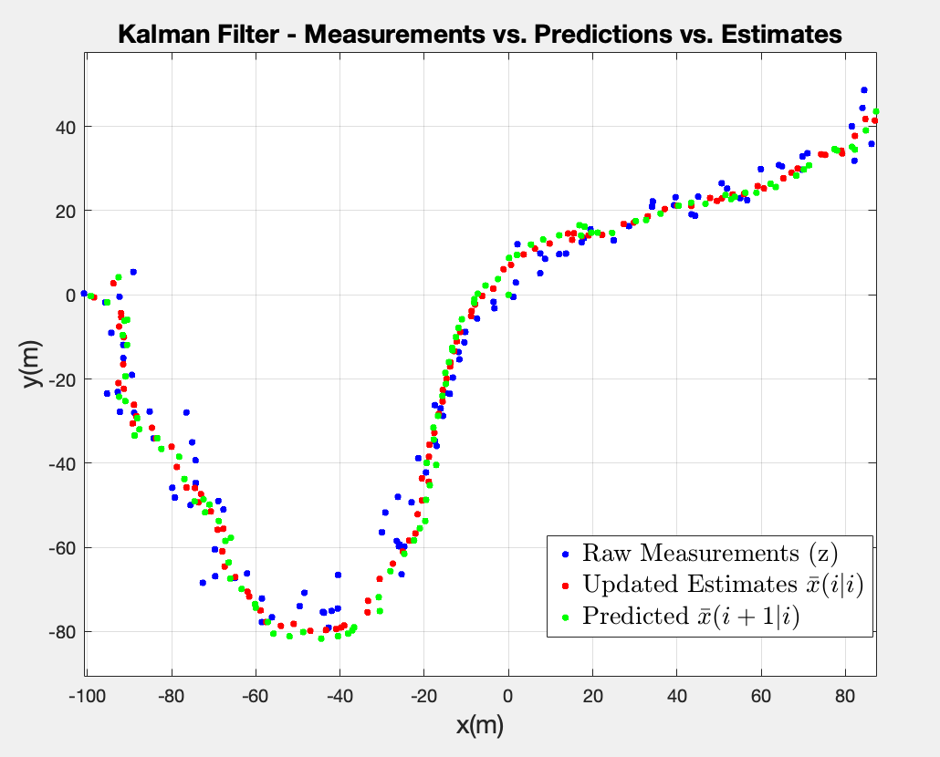
From the Figure above, I can safely say that the raw measurements are the noisiest of the bunch, and it’s expected since they represent measurements with real noise. In theory, the predicted positions should be less noisy but prone to drift since they rely entirely on the system’s kinematic model and the previous state estimate without incorporating current real-world observations and the estimated (updated) positions should be the smoothest sequence because the Kalman Filter optimally weights and combines the noisy measurements with the kinematic predictions.

However, the difference in this plot between the predictions and the estimates is very subtle. I would argue that the predictions have the smoothest shape geometrically since they rely more on the proposed kinematic model and the updated estimations are a little bit more noisy since they take those real-world observations and weigh them in the final results, which slightly contradicts my earlier statement regarding theory. One reason I could think of is the fact that the measurement noise covariance matrix $C_n$ is relatively large when compared to the process noise, so the Kalman Gain K is small and the filter trusts the prediction more than the measurement. This means the update step barely moves away from the prediction, hence they look almost identical in the plot.

---

4. Add the uncertainty regions. What are your observations w.r.t. the shape and size of the ellipse depending on $i$? Plot for every 3 iterations.

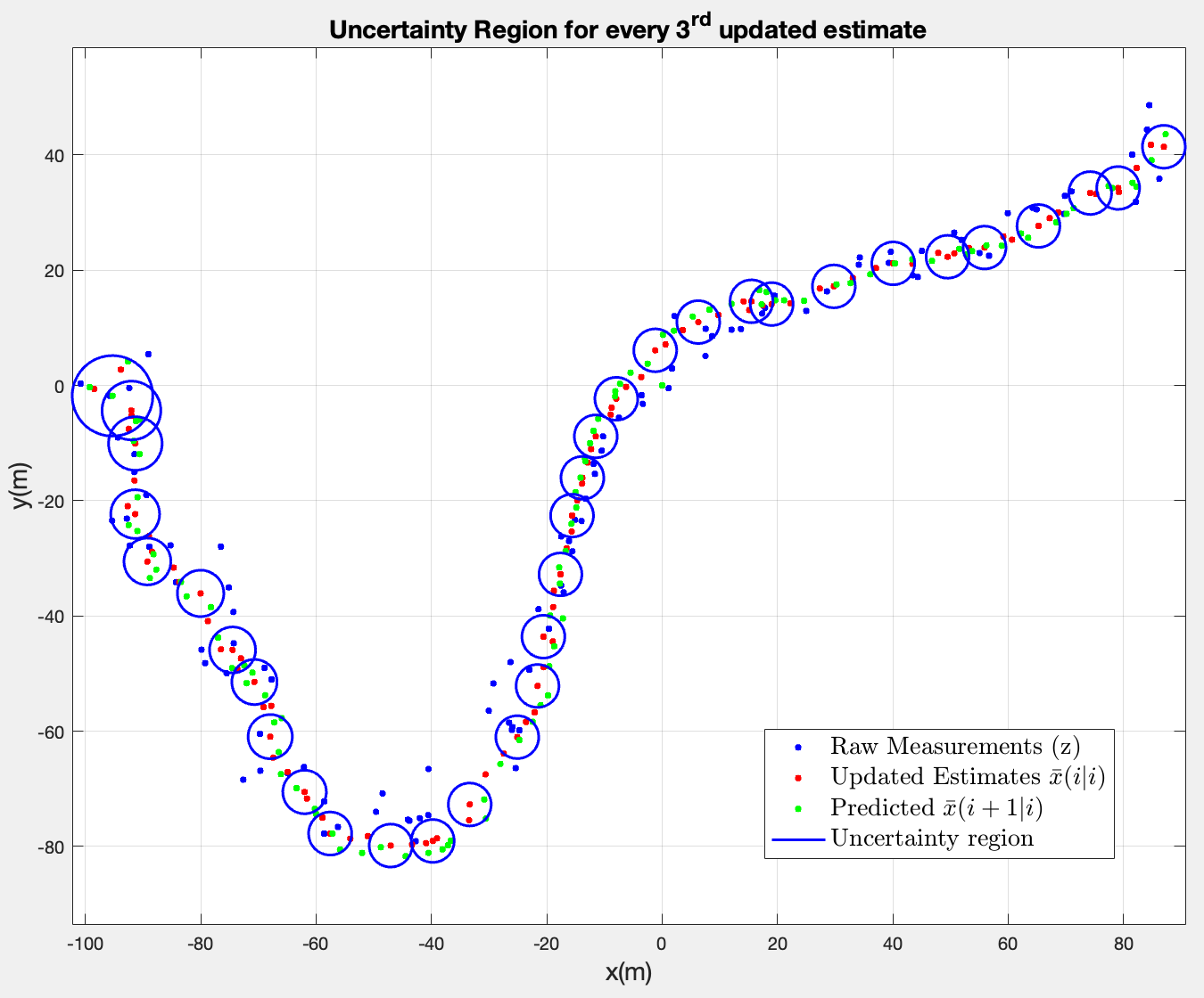
First impression is rather interesting. All uncertainty regions are circles, which corresponds to the diagonal shape of $C_n$, which suggests that the measurement noise is equal in both $x$ and $y$ directions i.e. symmetric.

It also seems they converge to a constant size after a few iterations. At the start, $C(0\mid -1)$ is large (high initial uncertainty), so the first few ellipses are big. Since the system is linear time-invariant, the filter progressively reduces uncertainty until the error covariance matrix $C(i\mid i)$ converges to a fixed value where the uncertainty added by $C_w$ at each prediction step is exactly balanced by the uncertainty removed by each update step.

---

5. Rerun Questions 2-4 while using the dlqe function to extract the Kalman Gain matrix and the covariance matrices of the steady state solution. Compare the matrices, to what extent to they agree? Compare and explain.

When subtracting the last iteration of my solutions to those from dlqe, the results are on the order of $1e-6$, $1e-8$, which is essentially numerical precision. This would confirm that my Kalman Filter has converged towards the steady state solution.

After rerunning the 3rd and 4th questions, I get the following results:

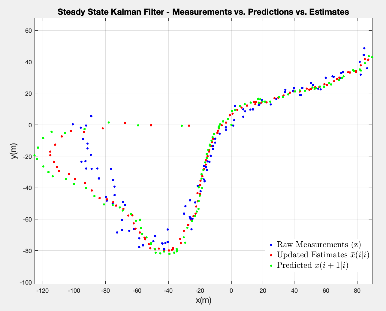
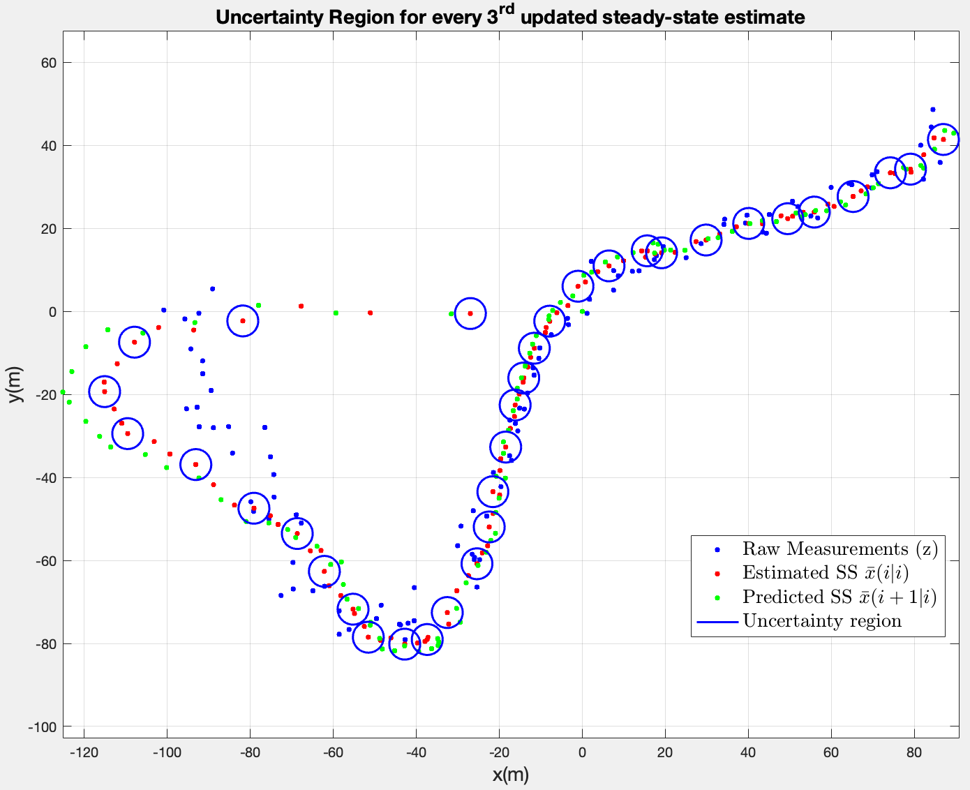
They suggest that the prediction and estimation start from the origin $(0,0)$, causing them to drift badly at the start. In retrospect, it does make sense: the initial uncertainty in the previous case was high, resulting the big ellipses. Here, the filter assumes it has already converged, without taking that initial uncertainty into consideration, so the steady state Kalman Gain $K_{ss}$ is too small to shift the results in the right direction.

In the previous case (time-varrying version), K started large because $C_{\mathbf{x}}(0)$ started large — initial uncertainty of 100 for the position. It translated into the filter trusting the initial radar measurements more.

The conclusion in this case is that the steady-state filter performs worse in the transient phase.