Prediction in a linear dynamic system

This is exercise 4/8 from my optimal estimation course. The focus is on propagation of uncertainty and prediction.

Context

Again, to gather data, we use dead reckoning. The navigator uses a log to measure the speed of the vessel and a compass to determine the heading. Together, they can be used to extract the velocity $v$.

• Consider $\hat{\xi }(i)$ an estimate that is available for position $\xi (i)$ and $v(i)$ the velocity determined at time $i$.
• Together, $\xi (i)$ and $v(i)$ provide sufficient information to deduce an estimate of the position valid for time $i+l$. So we call $\hat{\xi }(i+l)$ the prediction with a lead of $l$ i.e. $l$-step ahead prediction.

So I want to develop a predictor that can predict the position of the ship and that provides an uncertainty region. So in this application, the mean and the covariance will be propagated in time as opposed to Fundamentals of parameter estimation - Part III, where they were static. And the whole application was static.

I am provided with the identified linear state space model

$$\{\begin{array}{rl}v(i)& =\xi (i+1)-\xi (i)\\ a(i)& =v(i+1)-v(i)\\ a(i+1)& =F_{1}a(i)+w_1(i)\end{array}$$

where $F$ is a time invariant system matrix, and $w(i)$ is a white sequence of Gaussian random vectors with zero mean and a time invariant covariance matrix $C_w$.

Invariant means they do not change over time. Now I’m a lil’ bit confused, I thought I would have dynamic parameters now. So it’s the states that change over time and not the params? Reading this again, ofc that’s what it means; that’s exactly what a dynamic system is, dumbo.

so the state space is of type

$$\mathbf{x}(i+1)=F\mathbf{x}(i)+w(i)$$

Like any shitty dead reckoning which I don’t support, velocity and position are obtained through integration of their respective derivative. I guess she said white noise so maybe not so bad if accumulated but still bad you know what I mean? I want a beer.

These equations hold only for dt=1. In continuous time:

• $v(t)=\partial \xi /\partial t$
• $a(t)=\partial v/\partial t$

In discrete time with sampling period $\Delta t$:

• $v(i)=(\xi (i+1)-\xi (i))/\Delta t$
• $a(i)=(v(i+1)-v(i))/\Delta t$

So integration becomes. Mind that $\Delta t=1$ and that’s it.

• $\xi (i+1)=\xi (i)+\Delta t\cdot v(i)$
• $v(i+1)=v(i)+\Delta t\cdot a(i)$

Questions

1. Using the first two state space equations, determine the matrix $F$ and the covariance matrix $C_w$. Use the xsi array (load mat) to deduce the $6\times (N-2)$ state vector $\mathbf{x}(i)$.

By focusing on extracting the next state (updates), I can simply rewrite

$$\mathbf{x}(i+1)=\{\begin{array}{rl}\xi (i+1)& =\xi (i)+v(i)\\ v(i+1)& =v(i)+a(i)\\ a(i+1)& =F_{1}a(i)+w_1(i)\end{array}$$

Clarification: The 3 dimensions are all 2-dimensional vectors representing the $x$ and $y$ axes. Because of this, the next time step requires $2\times 2$ identity matrices, moving the overall system matrix $F$ to $6\times 6$.

so, according to the equations above, $F$ and $C_w$ should look like this ($\xi$ | $v$ | $a$).

$$F=\left[\begin{array}{c}{I}_2{I}_2{O}_2\\ O_2{I}_2{I}_2\\ O_2{O}_2{F}_1\end{array}\right]$$ $$C_w=\left[\begin{array}{c}{O}_2{O}_2{O}_2\\ O_2{O}_2{O}_2\\ O_2{O}_2{C}_{w_1}\end{array}\right]\text{ with }w(i)=[0,0,w_1(i){]}^T$$

Some explanations to myself

The overall system covariance matrix would suggest that uncertainty enters the system only through the acceleration. Position and velocity accumulate that uncertainty over time, but they don’t have their own independent noise sources. I feel like this is wrong from the start since it assumes the position and velocity are perfectly determined by integrating acceleration.

• Both $F$ and $C_w$ consider the $[{\xi }_{\mathbf{x}},{\xi }_y,v_{\mathbf{x}},v_y,a_{\mathbf{x}},a_y{]}^T$ vector.

---

2+3. Suppose we start from i=10 (11 in MATLAB because of 1-indexing). Predict the position at time j=i+l, where l=90. In other words, using $\mathbf{x}(10)$, I want to predict the position $l=90$ steps ahead $\hat{\mathbf{x}}(j\mid i)$. The prediction equals only the expectation i.e. don’t take the covariance into consideration.

I think the idea is self explanatory. I need to apply $\mathbf{x}(i+l)=F\mathbf{x}(i)$ over and over again until I will have hit the target. However, it says in the context that $\mathbf{x}(i+l)$ is based on measurements taken at time $i$. It means that I never update $\mathbf{x}(i)$ i.e. it’s fixed.

The covariance is 0 at time $i=10$ and so on because the question says it is considered exact.

So bottom line, just keep applying $F$ forward. No updates, pure prediction.

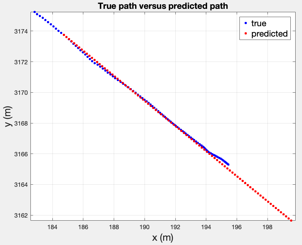
The results suggest:

1. If we only predict and never update, we never react to the turn around the end. Also, the scales are different and the prediction assumes a mostly constant step at every iteration (See $F$, I have $I_2$ for position).
2. The prediction is a straight line, since propagating through $F$ is linear.

---

4. Suppose that the covariance matrix of a prediction $\hat{\mathbf{x}}(j\mid i)$ is denoted by $C(j\mid i)$ i.e. the covariance matrix of the prediction error $\hat{\mathbf{x}}(j\mid i)-\mathbf{x}(j)$. Draw the ellipse associated with the submatrix $C(j\mid i)$ for $\hat{\xi }(j\mid i)$.

From the book (page 90):

The white noise indicates that the expectation is zero and the autocorrelation is governed by the Kronecker delta function:

$$\mathbb{E}[w(i)]=0,$$ $$\mathbb{E}[w(i)w^T(j)]=C_w(i)\delta (i,j)$$

• $C_w(i)$ is the covariance matrix of $w(i)$.

In the special case, where neither $F(i)$ nor $C_w(i)$ depend on i (i.e. the state space model is time invariant), $\dots$ the sequence $C_{\mathbf{x}}(i),i=0,1,\dots$ converges to a constant matrix. If such is the case, then:

$$C_{\mathbf{x}}=F{C}_{\mathbf{x}}{F}^T+C_w(4.14)$$

• This is the discrete Lyapunov equation

---

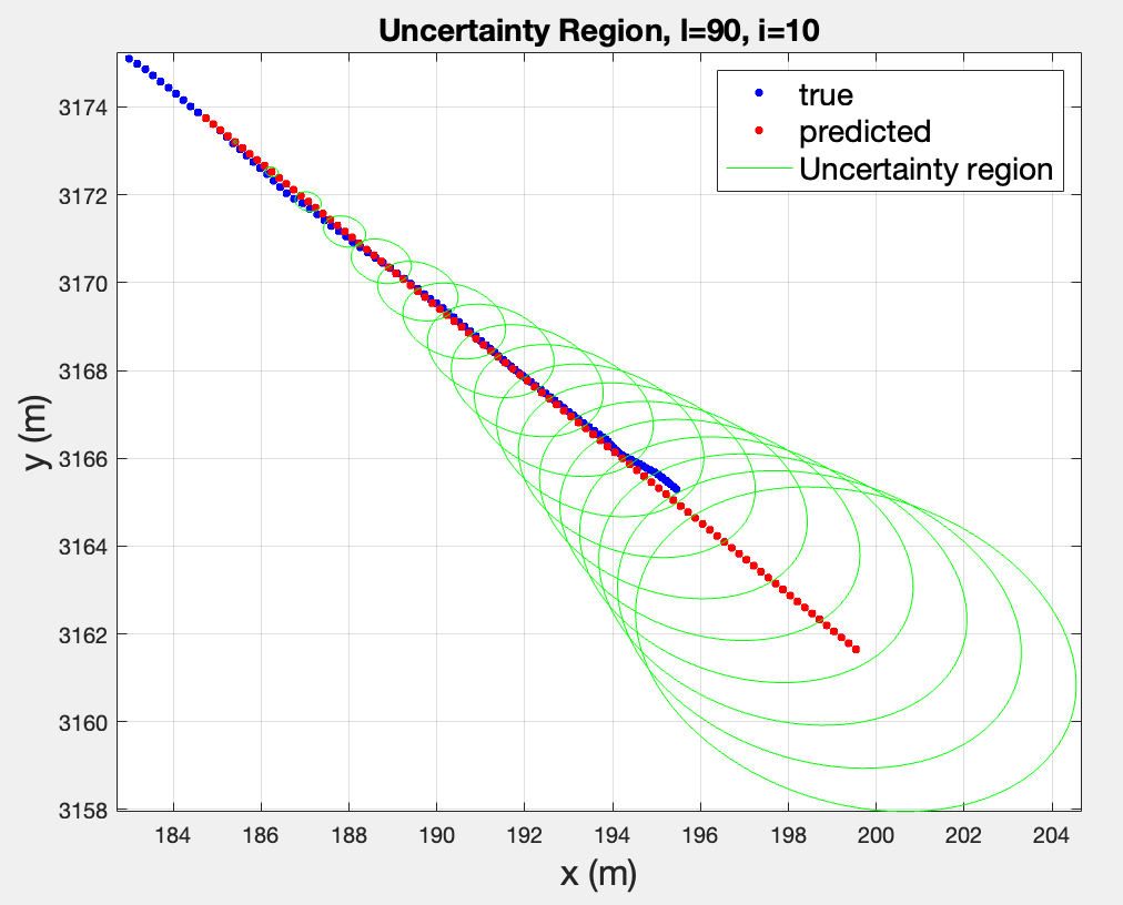
**5. Repeat for $i=30,50,70,90$ and $l=70,50,30,10$. j is fixed at 100. Explain the results.

I plotted the uncertainty region for every 5 steps.

The trends reveal a obvious pattern: the larger the lead, the larger the uncertainty regions. This is expected, since every step adds $C_w$ to the covariance, so the longer I predict without updating, the more uncertainty accumulates.

For mostly every case, the true path eventually diverges outside the ellipses, especially in those where the prediction took place before the turn.

Bottom line: this is pure dead reckoning without any new measurement updates. The shorter the lead, the more reliable the prediction.