Particle Filtering

So I need to finish my notes on the Particle Filter. The process is the exact same as in the EKF application.

Sections 4.4 and 9.3.3 from the book.

Two differences from the prior exercise

1. The intended heading ${\varphi }_0(i)$ is now time variant and given at any moment in time. The equation also stays the same, but ${\varphi }_0$ is not constant anymore. It translates directly in the control input ($u$) vector changing every iteration.
2. We now assume at time $i=0$ a position variance of ${\sigma }_{{\xi }_{\mathbf{x}}}={\sigma }_{{\xi }_y}=100m$ instead of $10000m$

Context

Apparently, the struggle shifts to expressing how consistent is the Particle Filter and how to measure it. So what we want is an equivalent to the NIS, but for the Particle Filter.

The idea is as follows:

Suppose that, using all previous measurements $Z(i-1)$ up to time $i-1$, the probability density of the state $\mathbf{x}(i)$ is $p(\mathbf{x}(i)\mid Z(i-1))$. Then, the probability of $z(i)$ is:

$$\begin{array}{rl}p(z(i)\mid Z(i-1))& ={\int }_{\mathbf{x}}p(z(i),\mathbf{x}(i)\mid Z(i-1))d\mathbf{x}\\ & ={\int }_{\mathbf{x}}p(z(i)\mid \mathbf{x}(i))p(\mathbf{x}(i)\mid Z(i-1))d\mathbf{x}\end{array}$$

Which makes total sense, looking at it?

• $p(z(i)\mid \mathbf{x}(i))$ is simply the model of the sensory system.
• $p(\mathbf{x}(i)\mid Z(i-1))$ is represented by the predicted samples.

The filter is consistent only if the sequence of observed measurement $z(i)$ obeys the statistics prescribed by the sequence of densities $p(z(i)\mid Z(i-1))$.

So the problem will be tackled by treating each scalar measurement separately ⇒ for each individual measurement element $z_n(i)$, we consider the hypothetical probability density $p_n(z,i)=p(z_n(i)\mid Z(i-1))$, i.e. the pdf of $z_n(i)$ given all previous measurements.

The cumulative distribution of $z_n(i)$ is then:

$$F_n(z,i)={\int }_{\infty }^z{p}_n(\zeta ,i)d\zeta$$

We now denote $u_n(i)\stackrel{\mathrm{def}}{=}{F}_n(z_n(i)\mid i)$ as test variables for each measurement element. It can be proven that if the particle filter behaves consistently, then the variables $u_n(i)$ are uniformly distributed between 0 and 1.

The consistency check boils down to testing whether the set $u_n(i)$ indeed has such a uniform distribution.

• In literature, the statistical test of whether a set of variables has a given distribution function is called a goodness-of-fit test.
• Algorithm 9.1 in the book

However, we’ll just use plots of the test variables to assess the consistency.

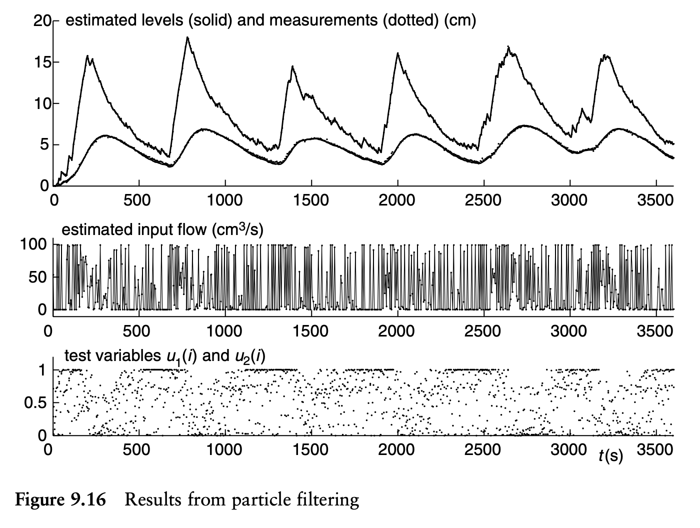
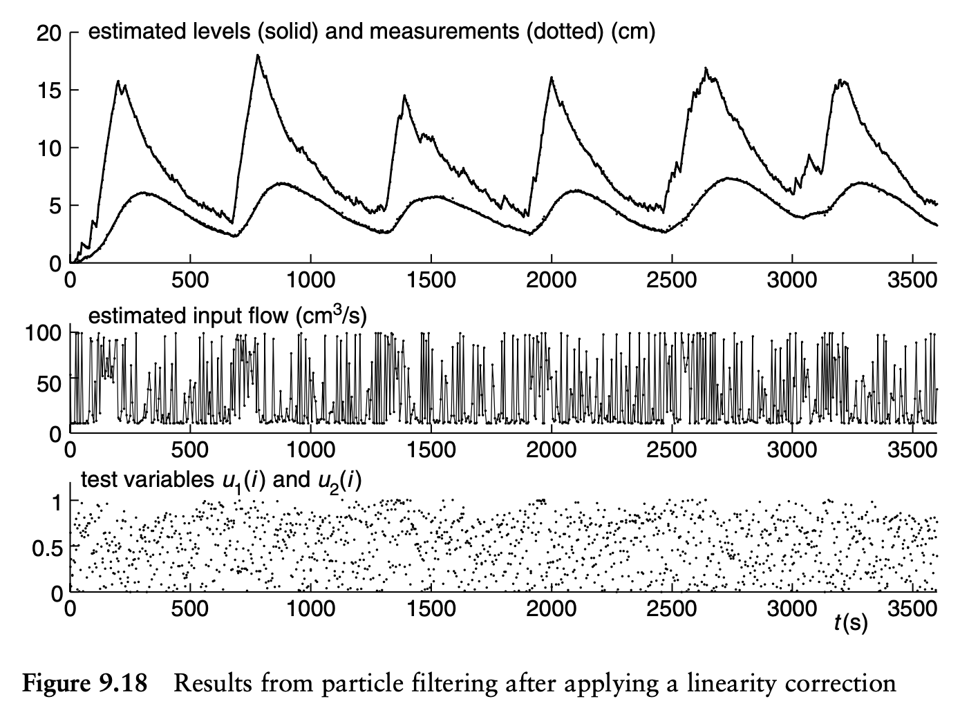
Another variable of interest is the number of particles. This variable can be used to see whether the normalized weight factors are evenly distributed.

$$K_{\text{eff}}(i)=\frac{1}{{\sum }_{k=1}^K(w_{\text{norm}}^{(k)}(i){)}^2}$$

• $K_{\text{eff}}=1$ is an extreme case indicating that only one weight factor is nonzero.

---

Questions

1. Implement the Particle Filter. Using the particles, calculate the MMSE estimate ${\hat{\mathbf{x}}}_{\text{MMSE}}(i)=\bar{\mathbf{x}}(i\mid i)$, and create a plot of the estimated path.

Assuming a Gaussian Distribution, the weights are calculated as:

$$w^{(k)}\propto \text{exp}(-\frac{1}{2}(z(i)-x^{(k)}{)}^T{C}_v^{-1}(z(i)-x^{(k)}))$$

• it says proportional because normally there should be a constant multiplied with the exponential. But since the weights are going to be normalized anyway, we can ignore it.
  • To normalize, we simply divide by the sum of the weights vector.

A Monte Carlo simulation uses a set of random samples generated from a known distribution to estimate the expectation of any function of that distribution. The first step starts with drawing $K$ samples from the prior probability density $p(\mathbf{x}(0))$.

• The mvnrnd function in MATLAB takes care of this.

The update step looks pretty much similar to the EKF; the main difference consists in computing the normalized weights and performing the Resampling by selection process presented in Section 4.4.2. The purpose is to delete samples with low weights, and to retain multiple copies of samples with high weights (without it, the filter can degenerate).

• After computing the cumulative sum of the weights vector by utilizing the $w_{\text{cum}}^{(k)}={\sum }_{j=1}^k{w}_{\text{norm}}^{(j)}$ equation (cumsum in MATLAB), I need to generate a random number $r$ uniformly distributed in $[0,1]$ and find the smallest $j$ such that $w_{\text{cum}}^{(j)}\ge r^{(k)}$ and then reselect the particles from that index $j$.
• For this part, I will simply search iteratively for j. I understand that using the golden rule is much more efficient, as the problem shifts to solving $w_{\text{cum}}^{(j)}-r=0$, but I want it to make sense to me.
  • My method would be $O(N^2)$, while my teacher’s approach would decrease the complexity to $O(N\log (N))$. However, my number of particles will be only 1000, so it should not affect the performance that much. Just keep in mind for future purposes.
  • I used the teacher’s method in the end :))

After resampling, don’t forget to reset the weights. It’s basic intuition: I’ve already used the weights to decide how many times each particle is copied.

I observed that by passing $C_n$ in the hmeas function, I get a smoother plot. Apparently, the explanation is that the filter trusts the measurements less, and that's why.

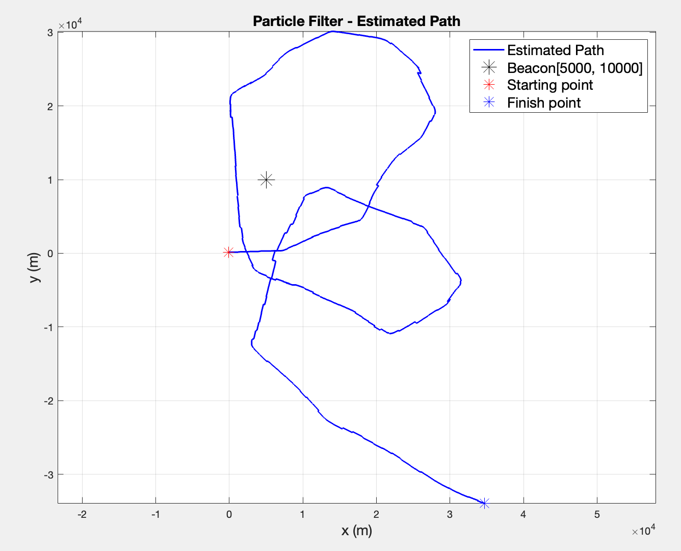
It doesn’t necessarily look wrong, but initially I expected a trajectory that resembled the EKF more. Since I did not necessarily have the intuition to tell whether the trajectory is right or wrong, I fell back to comparing the intended thrust ($t_0$) and the estimated thrust ($7^{th}$ column of ${\mathbf{x}}_{\text{MMSE}}$) and the intended headings (fi0 array) with the estimated headings ($8^{th}$ column of ${\mathbf{x}}_{\text{MMSE}}$).

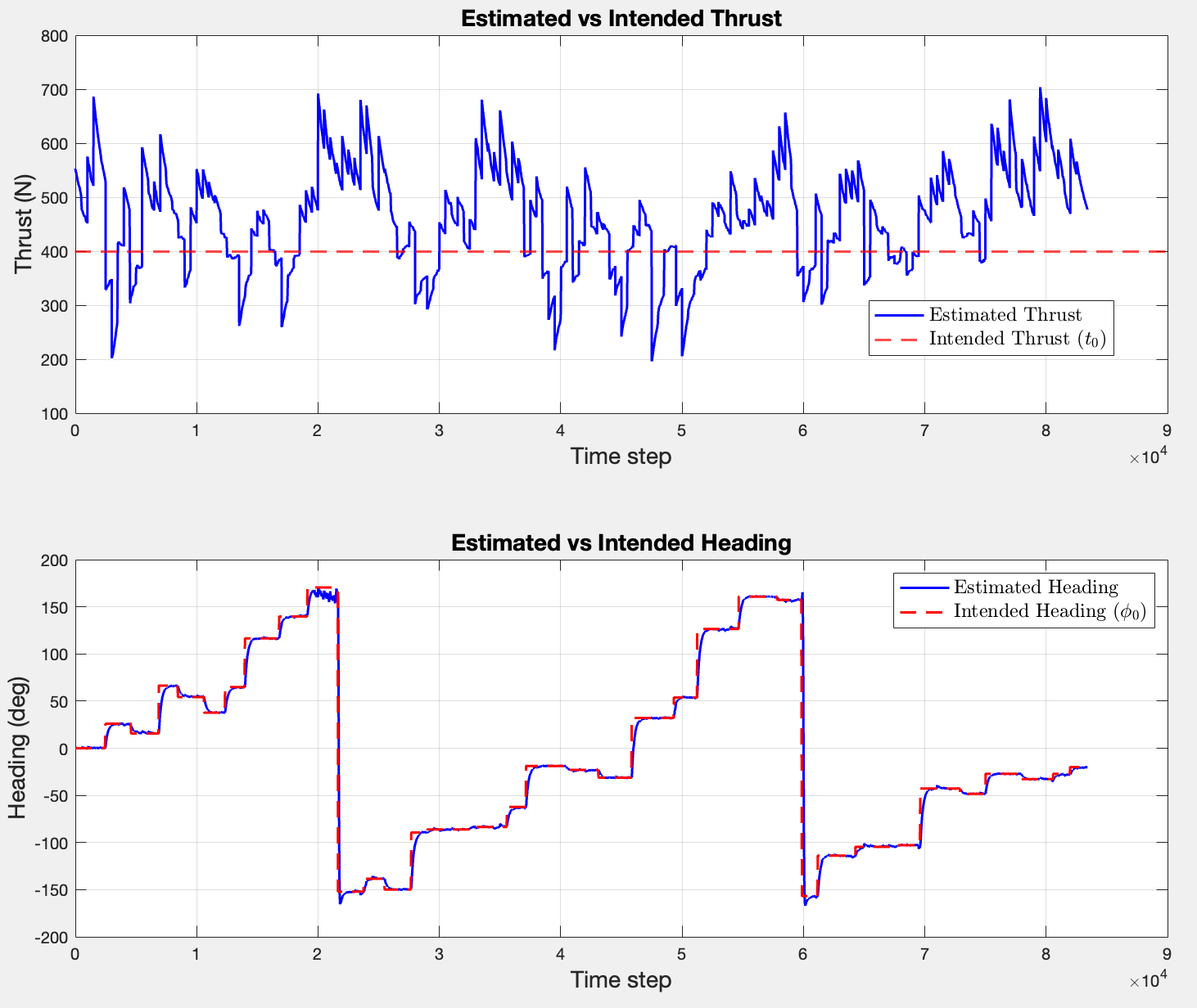
These comparisons would suggest that the filter successfully follows the input action vector, which confirms that the implementation is correct. Regarding the estimated thrust, the mean of the estimated vector is ~460N, which implies that the filter is actively trying to reach the intended 400N. The almost 1:1 comparison of the headings is, however, the final argument that the presented trajectory is indeed correct.

---

2. Extend the code such that a covariance matrix is calculated at each measurement step. Plot the uncertainty regions.

According to the Lectures, the covariance matrix is defined as

$$C_{\mathbf{x}}=\sum _{k=1}^K{w}^{(k)}({\mathbf{x}}_s^{(k)}-\bar{\mathbf{x}})({\mathbf{x}}_s^{(k)}-\bar{\mathbf{x}}{)}^T$$

My intuition tells me that I could discard the weights vector since I resample them to a unit distribution after the update, and the information would have already been saved in the current estimate anyways, since ${\mathbf{x}}_{\text{MMSE}}(k)=\mathbf{g}({\mathbf{x}}_s^{(k)})\cdot w^{(k)}$, i.e. particles * weights. So in the end, I can simply calculate $C_{\mathbf{x}}=\text{deviations}\cdot \text{deviations’}/\text{No\_particles}$.

---

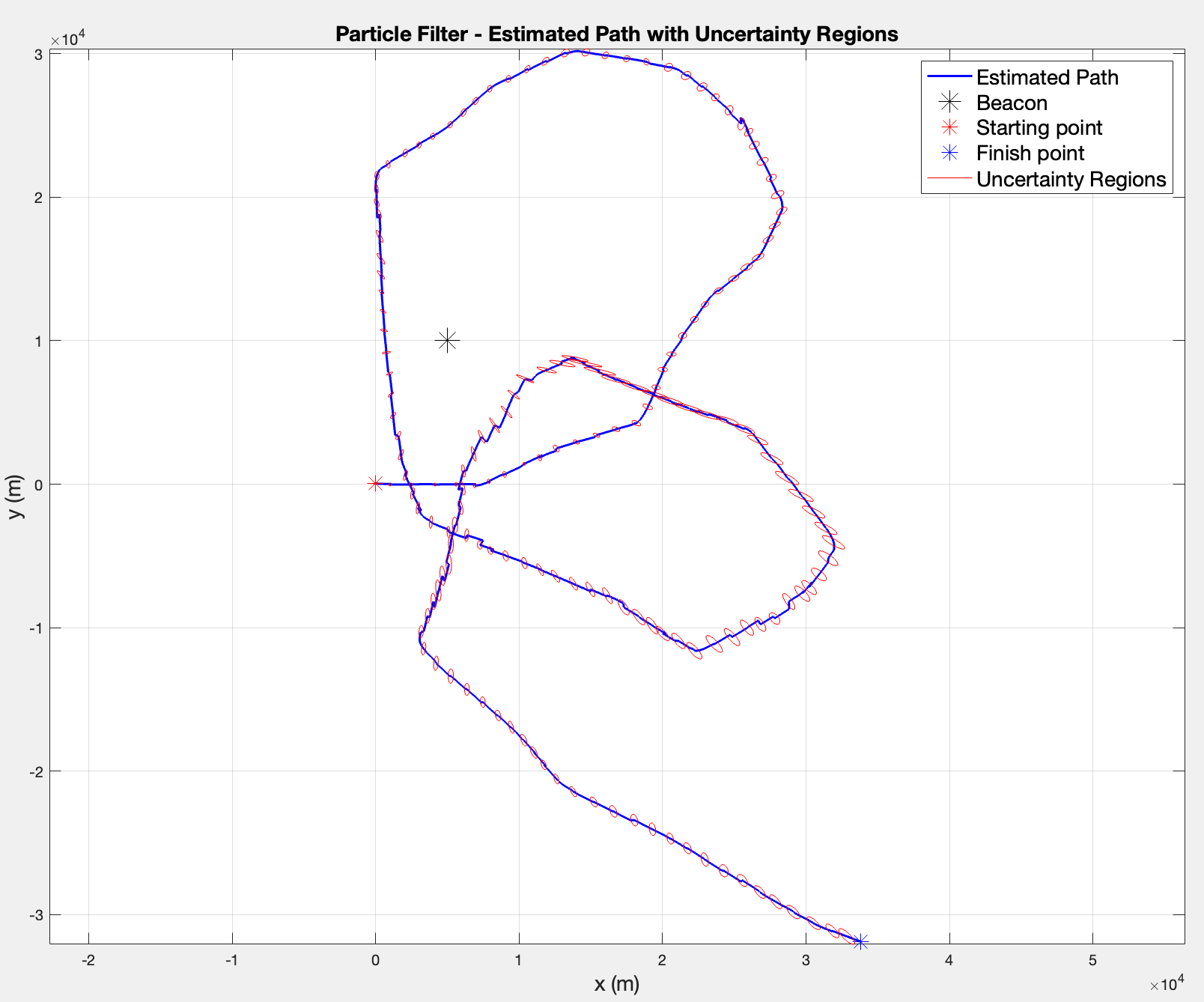
3. Extend the code such that the test variables $u_n(i_m)$ are calculated. Plot them and interpret the results.

I provided context on the test variables above. According to Listing 9.10 from the book, I can simply adapt the calculations to what I have by counting how many predicted samples fall below the actual measurement, which directly approximates $F_n(z_n(i)\mid i)$.

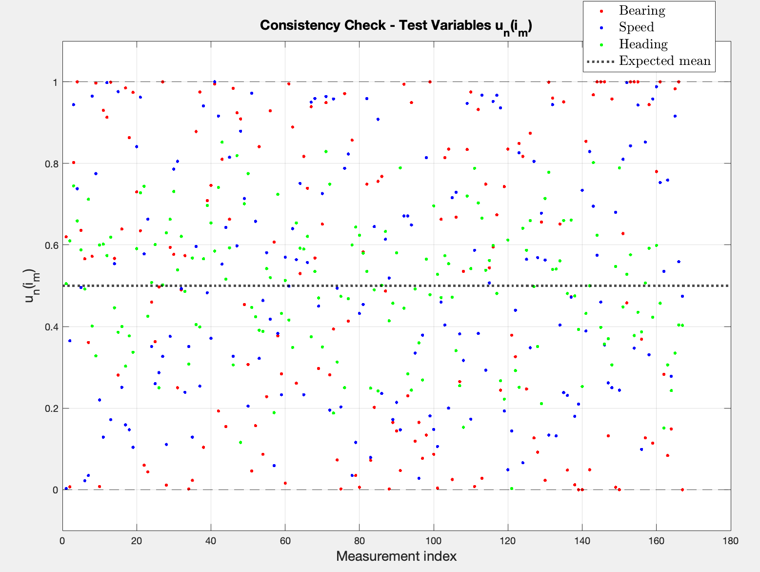
The plot reveals no obvious trends and consistency. In terms of heading, it seems like the values are more centered which would suggest the particles don’t spread much in heading space between updates, which correlates with the earlier plot that showed the 1:1 characteristic. However, Bearing and Spped seem to uniformly distributed in $[0,1]$, with no visible bias. Moreover, all variables seem to be symmetric around the expected mean of 0.5, which is exactly what we hoped for.

In conclusion, this consistency check reveals that the particle filter is consistent for all three measurement channels, i.e. the filter’s predicted probability densities $p(z(i)\mid Z(i-1))$ correctly describe the actual distribution of measurements. It further translates into a good choice of the modeled noise $C_w,C_n$, unlike in the EKF case.

---

4. Calculate the effective number of particles after each measurement. Plot this variable and explain the results

In the context I mentioned that this is another variable of interest since it reveals whether the normalized weight factors are evenly distributed.

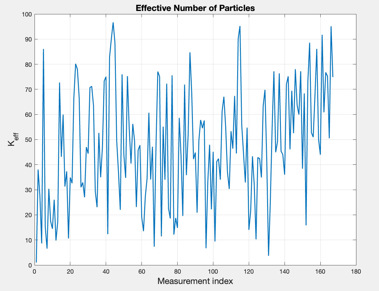
The Figure above represents the constantly changing number of effective number of particles for an initial number of 1000 particles. It reveals a mean value of ~47 effective particles out of 1000. This translates to the particle weights being extremely uneven - only a small fraction of the particles are actually contributing to the estimate at each measurement update.

---

5. Perform some experiments such that you are sure that you have a sufficient number of particles

After running the script for different values of No_particles, I got the following Table and Figure:

Number of Particles	Mean Value of K_eff
100	5.9934
1000	47.6997
2000	93.5558
3000	134.8896
4000	187.6875
5000	230.3501
10000	463.9912

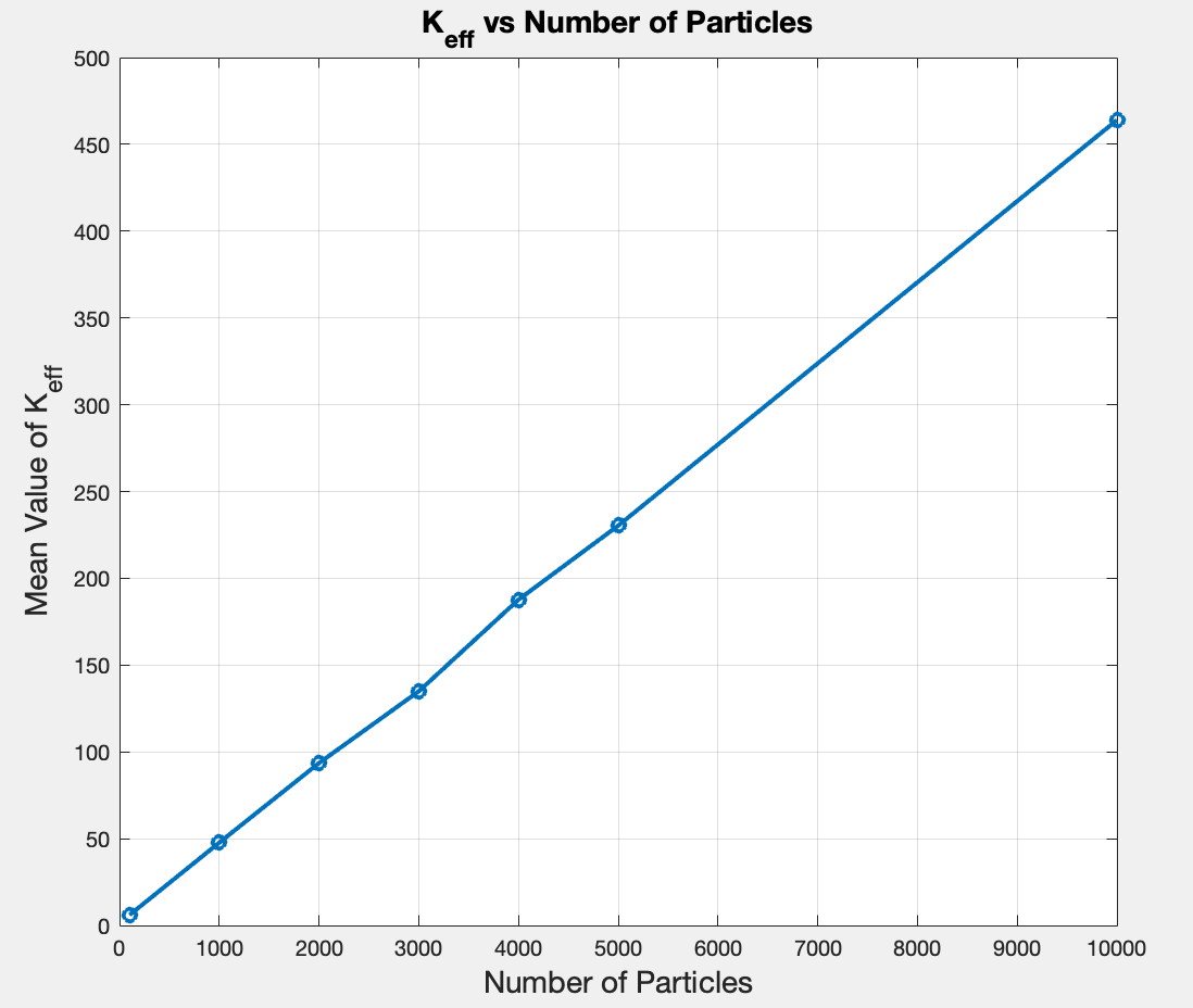
They reveal an obvious linear trend, with the mean staying around 4-5% of N regardless of how many particles I use. Since adding more particles doesn’t change this ratio, it could mean that the measurement is consistently informative enough, but that would be an educated guess.

The question asks how I am sure whether I have sufficient particles. I would argue the important aspect is for the posterior to be well represented. One area where I visibly see obvious changes is the representation of the uncertainty regions, which become more clear as $N$ increases.

For example, the Figure below is a comparison for $N=1000$ (left) and $N=5000$ (right)

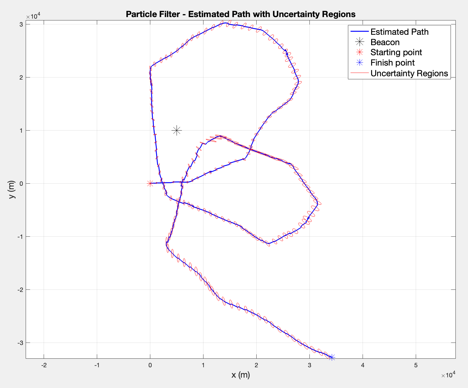
Since the right plot ($N=5000$) shows smoother ellipses and a more consistent path, particularly in the complex crossing regions near the center, I would consider that $N=5000$ gives a better posterior representation and has a reasonable amount of effective particles (~230).

---

6. Adjust the EKF code to anticipate the time variant $\varphi$ vector. Interpret the results regarding the path + uncertainty regions, as well as the plot of the NIS.

Analysis of the path and the uncertainty regions

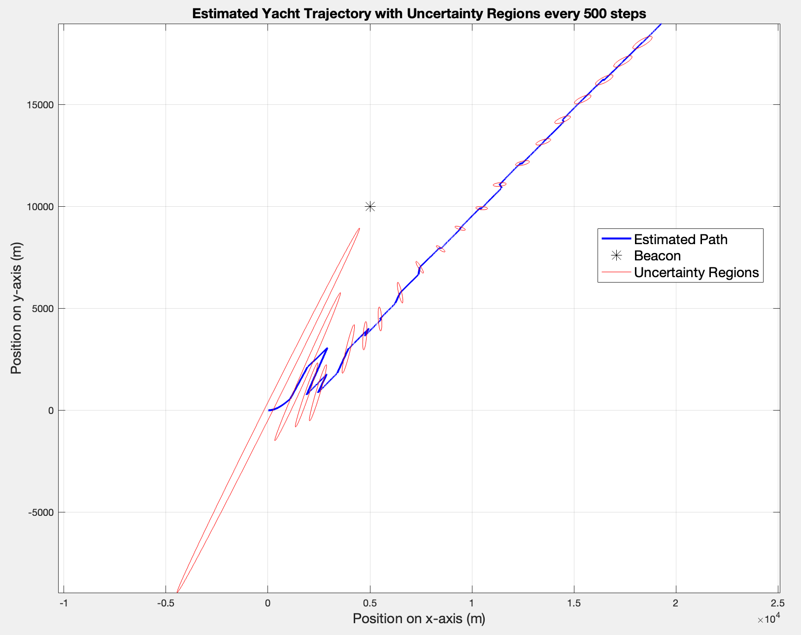
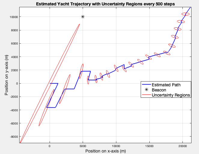
The right plot (time-variant ${\varphi }_0$) shows a much clearer path with sharp turns and clear directional changes. The right path (fixed ${\varphi }_0=45deg$) shows the yacht drifting mostly in one direction diagonally, which does make sense since a constant heading of $45deg$ simply drives the yacht in that direction indefinitely.

In terms of uncertainty regions, both cases display large initial uncertainty that shrinks as measurements update the states. However, it seems that the time-variant ${\varphi }_0$ has larger ellipses which makes sense since the yacht is constantly changing direction, so between measurements he kinematic model is less certain about where the yacht might be next. The time span between two updates remains 500 seconds.

Analysis of the NIS Scores

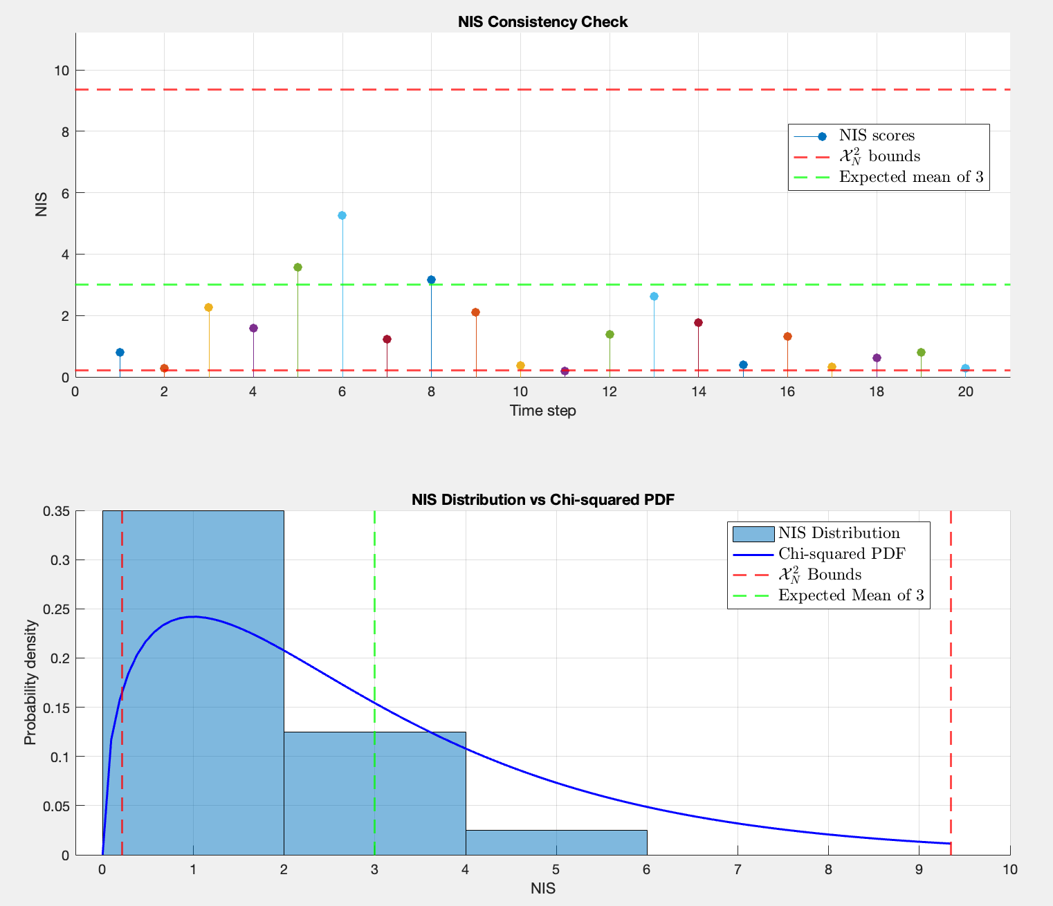
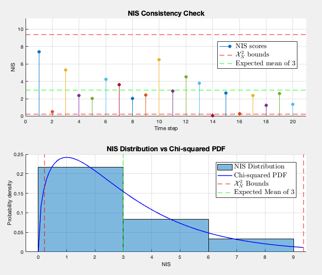
The time-variant ${\varphi }_0$ gives a mean NIS of 2.9 versus 1.51 for fixed ${\varphi }_0$. The new performances seem nearly perfect, since the mean NIS should be ~3 (DOF) for a consistent filter. In the previous case, the filter was overly pessimistic. This shifts the idea that $C_w,C_n$ were wrong; now they seem to be correctly tuned for the time-variant case.

Therefore, it seems that not the noise covariance matrices were the issue in the fixed ${\varphi }_0$ case, but the model itself. The NIS score is then not just a tool for tuning $C_w,C_n$, but also a model validation tool.

---

7. Which of the two estimation methods do you prefer? Motivate! Computational load is of secondary importance.

There are both upsides and downsides to both methods. For example, the EKF started showing good results when we introduced the time-variant ${\varphi }_0$, with the NIS indicating that the filter is approaching its ideal form. Moreover, from a visualization point of view, the EKF is able to compute the covariance matrix at each iteration, not only at measurement times as in the PF. Also, even for a non-linear system like this, the EKF was able to handle those non-linearities with some light assumptions/linearizations in a deterministic manner — running it twice will give the same result, while the PF introduces randomness through the particle sampling.

For the Particle Filter, the consistency check revealed ideal results, with all the variables being symmetric around $[0,1]$, which signals the correct distribution of measurements. The PF also makes no assumptions about linearity and works directly with the nonlinear model, which reveals a more truthful representation of the results, as close as possible to reality. Therefore, for highly nonlinear systems or different distributions than Gaussian, the PF is expected to perform better.

Having the advantages and disadvantages listed, I would personally choose the EKF for this specific application. It was able to handle the non-linearities through the selected assumptions and the representation with the time-variant ${\varphi }_0$ looked more than decent. Both methods give comparable consistency check scores, and the PF’s advantage of handling non-linearity fades since the posterior remains approximately Gaussian throughout (the posterior revealed clean ellipses regarding uncertainty regions, never a ‘cloud’). Part of my last arguments holds also because the measurements are informative and frequent enough - every 500 seconds, the posterior gets corrected on three measurement channels.

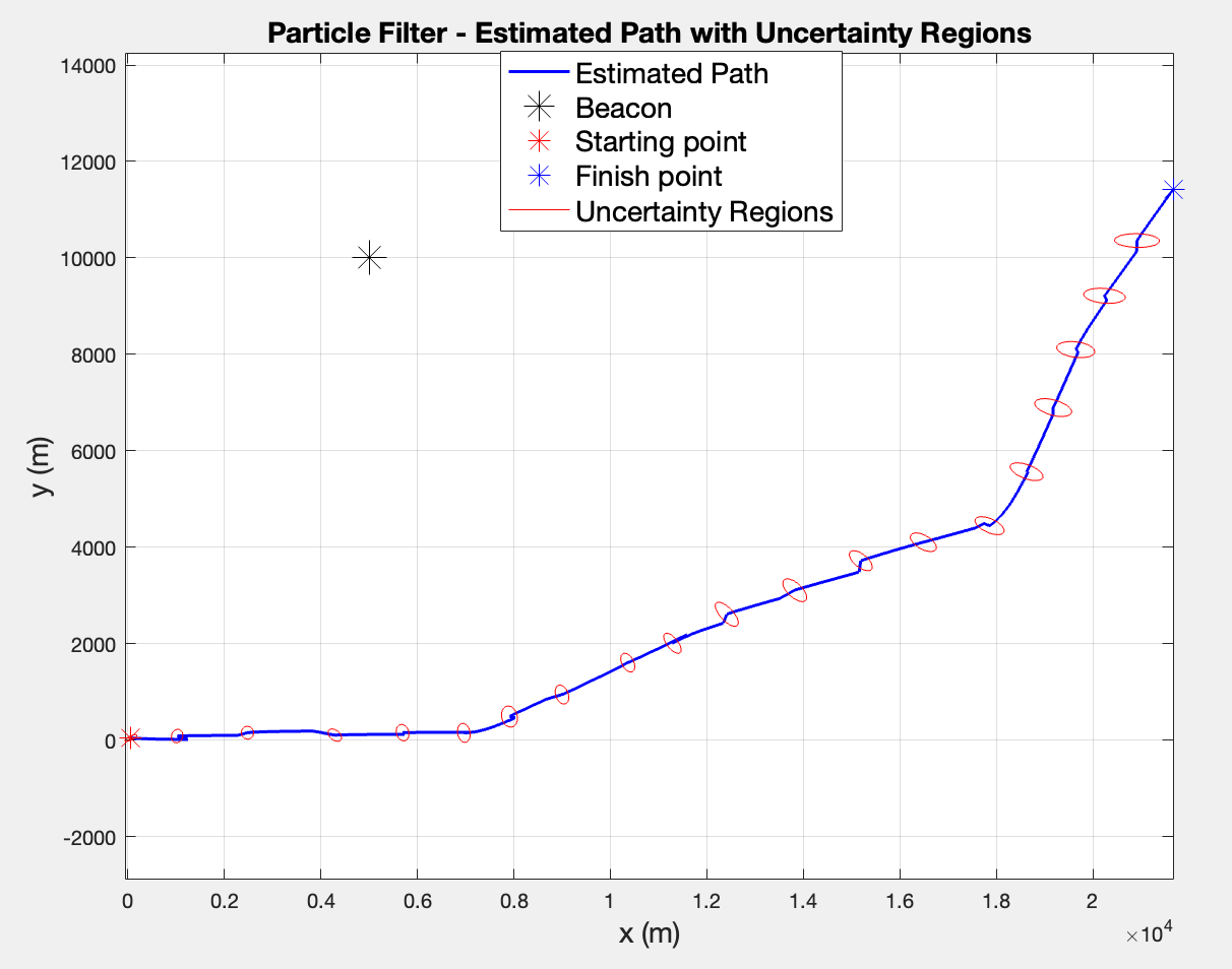
The plots reveal a trajectory and uncertainty region comparison between time-variant ${\varphi }_0$ EKF (left) and PF (right) for 10000 iterations.