Dimensionality Reduction

Start with Curse of Dimensionality.

Various approaches are possible:

• Feature Selection keeps only a subset of features.
  • There are $2^d$ distinct subsets of $d$ features.
• Clustering, Linear projection, Non-linear transformations, Similarity-based embeddings transform the features.

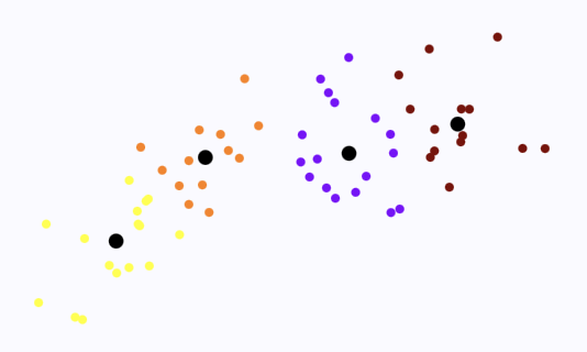
Vector Quantisation

Cluster the features and replace features by cluster ID. Since the number of clusters $<$ number of features, it results in dimensionality reduction.

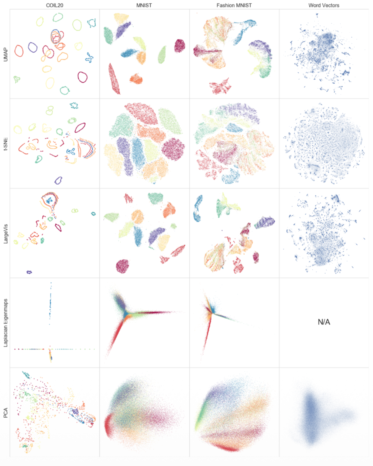
Small peek to how the following methods represent the data:

Linear Dimensionality Reduction

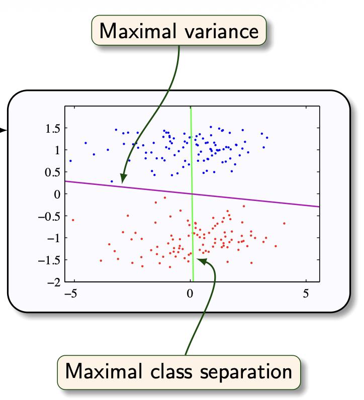
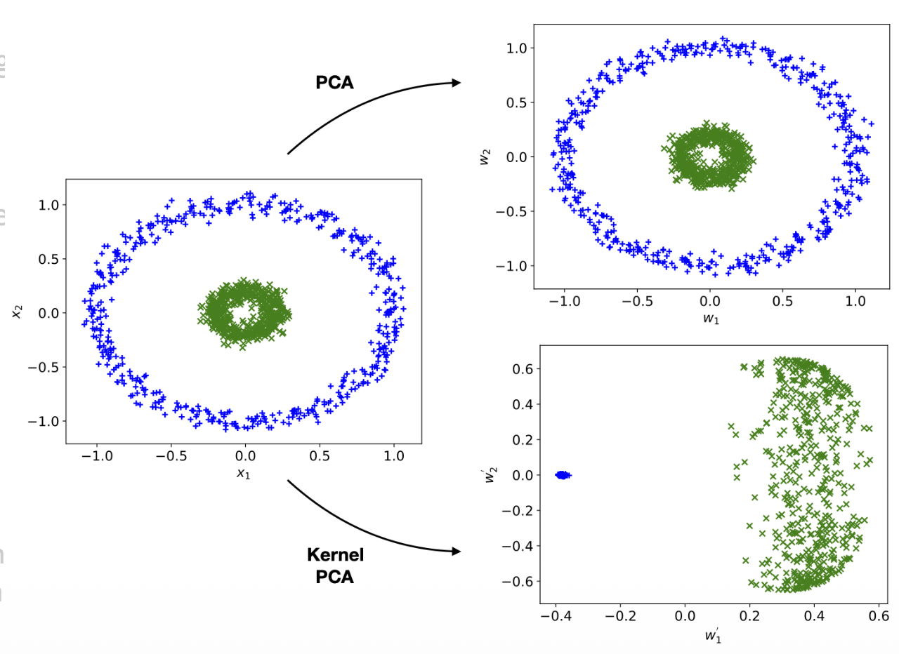
PCA is the most well-known method for dimensionality reduction. It does an orthogonal projection of the data into a lower-dimensional subspace, so that the variance of the projected data is maximised.

• Equivalently: linear projection that minimises the mean-squared distance between data points and their projection
• PCA can be used to normalize the dataset so as to make different dimensions decorrelated. (right)
• The maximal variance does not always correspond to optimal class separation (left)

One problem with this formulation of PCA is that the covariance matrix becomes huge as the dimensionality of the data increases.

• A $256\times 256$ image results in $65536\times 65536$ covariance matrix (which requires 48GB to store) — each feature relates to each other.

Probabilistic PCA or PPCA

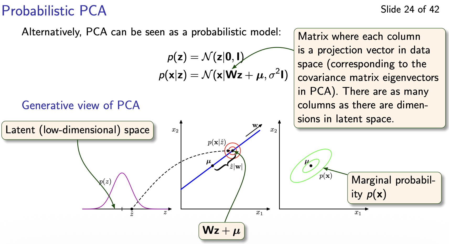
The probabilistic formulation of PCA is equivalent with PCA, but has several advantages:

• Gradient descent optimizes the model without computing the covariance matrix
• likelihood function allows direct comparison of different models.
• The model can be sampled from to generate new data and can be optimized despite missing data.

Nonlinear Dimensionality Reduction

We can replace the covariance matrix $\Sigma$ in PCA by a Gramm matrix $K$ from the Kernel Trick $\Rightarrow$ Kernel PCA.

• $K$ depends on all data; previously unseen data changes projection.

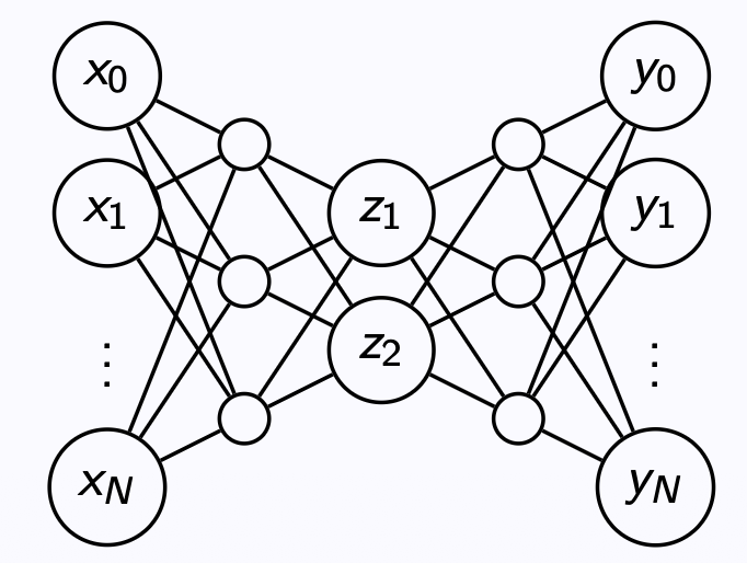
Autoencoders ensure same dimensionality between the input and the output, but its the latent space that forces compression. Adding hidden layers allows non-linear transformations.

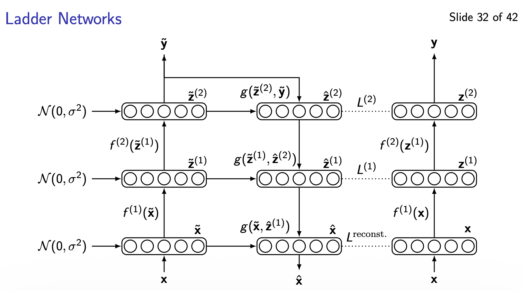
Ladder Networks de-noise at every layer of the auto-encoder-decoder & the loss is the weighted sum of all layer losses.

VAEs (Variational AutoEncoders) add a probabilistic twist. In theory, we can use Bayes’ theorem to compute $p(z\mid x)$. It can be approximated by sampling.

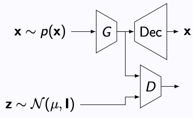
A standard GAN maps random noise to data space, pitting a generator against a discriminator that evaluates data samples. An AAE (Adversarial Autoencoder) couples a standard autoencoder with an adversarial network. In an AAE, the encoder acts as the generator, mapping data into an aggregated latent distribution, while the discriminator evaluates the latent code against an imposed prior distribution rather than inspecting real versus generated images.

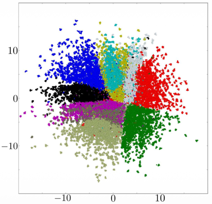
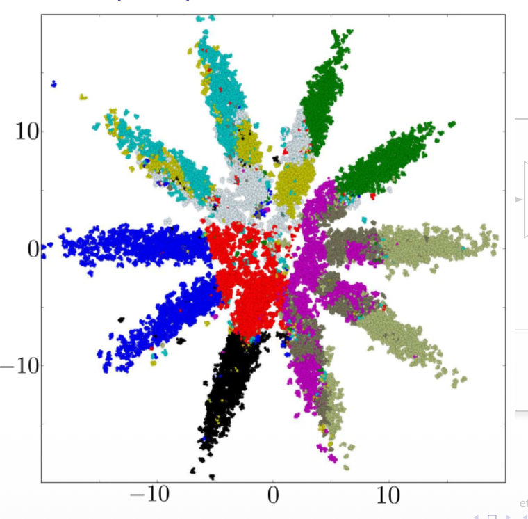
Both plots show the 2D latent space representations of MNIST test digits from the original Adversarial Autoencoders paper (Makhzani et al., 2015), comparing how different priors and training objectives shape the latent code $z$:

• The circular disk on the left is an AAE regularized against a standard single 2D Gaussian prior $\mathcal{N}(0,I)$. The adversarial discriminator forces the aggregated posterior $q(z)$ to uniformly fill the circular Gaussian density without holes or gaps between digit classes.
• On the right we have a model where the target prior is a mixture of 10 2D Gaussians arranged symmetrically around the origin. Because each Gaussian mode corresponds to a branch, the 10 distinct digit classes are separated along their respective radial modes.

Non-parametric Dimensionality Reduction

ML manifold $\approx$ smooth, low-dimensional subset of high-D space.

A manifold is a low-dimensional surface embedded in a higher-dimensional space. In Machine Learning, we often say that high-dimensional data (like images) lies on a low dimensional manifold.

Think: although an image has 1000s of pixels, the actual set of realistic images lives on a much smaller subspace.

Examples

• “Even though these images are 64x64, they really lie on a lower-dimensional manifold — maybe just 100 dimensions.”
• “The generative model learns to map random noise onto the data manifold.”

In order to model a nonlinear manifold, we can approximate the structure through a combination of linear models.

Combination of linear models

1. Cluster the data using K-Means and apply PCA to each group
2. Better: Use the reconstruction error for cluster assignment
3. Better still: Use mixture of PPCA. This provides a full probabilistic treatment and Bayesian treatment allows us to find the number of components automatically

Locally Linear Embedding

As an extreme case, we can represent each data element as a linear function of its $K$ neighbours.

$${\mathbf{x}}_i=\sum _j{w}_{ij}{\mathbf{x}}_j$$

• Optimize ${\sum }_i\left|{\mathbf{x}}_i-{\sum }_j{w}_{ij}{\mathbf{x}}_j\right|$ to find $w_{ij}$
• Create a representation $z$ in any dimensionality, while keeping $w_{ij}$ fixed, by optimizing

$$E(\mathbf{Z})=\sum _i\left|{\mathbf{z}}_i-\sum _j{w}_{ij}{\mathbf{z}}_j\right|$$

Pros:

• Efficient for large datasets
• Single parameter to tune $K$
• Scale-invariant, rotation-invariant, translation-invariant

Cons:

• Not useful for representing future data
• Can be unstable in sparse areas of dataset

t-Distributed Stochastic Neighbor Embedding (t-SNE)

t-Distributed Stochastic Neighbor Embedding (t-SNE) is a technique for dimensionality reduction that is particularly well suited for the visualization of high-dimensional datasets by mapping pairwise similarities into probabilities and matching them in a low-dimensional space

Basic idea of t-SNE

1. Pairs of points that are distant in the original space should be distant in the low-dimensional embedding. Pairwise Euclidean distances between points $x_i$ and $x_j$​ are converted into conditional probabilities using a Gaussian distribution centered at $x_i$:

$$p_{j|i}=\frac{\exp (-\Vert {\mathbf{x}}_i-{\mathbf{x}}_j{\Vert }^2/2{\sigma }_i^2)}{{\sum }_{k\ne i}\exp (-\Vert {\mathbf{x}}_i-{\mathbf{x}}_k{\Vert }^2/2{\sigma }^2)}$$

• To ensure symmetry and stabilize gradients, joint probabilities are defined as $p_{ij}=\frac{p_{i|j}+p_{j|i}}{2n}$

2. Pairs that are close by in the original space should be close in the embedding. In original SNE, the low-dimensional space also used a Gaussian distribution. t-SNE instead adopts a heavy-tailed Student-t distribution for low-dimensional coordinates:

$$q_{j|i}=\frac{\exp (-\Vert {\mathbf{y}}_i-{\mathbf{y}}_j{\Vert }^2)}{{\sum }_{k\ne i}\exp (-\Vert {\mathbf{y}}_i-{\mathbf{y}}_k{\Vert }^2)}$$

1. Optimization via KL Divergence. The low-dimensional coordinates $y$ are learned via gradient descent by minimizing the Kullback-Leibler (KL) divergence between $p$ and $q$.

• Because KL divergence places a heavy penalty on modeling close high-dimensional points ($p_{ij}$​ high) as distant points ($q_{ij}$​ low), the method strongly preserves local neighborhood structure.

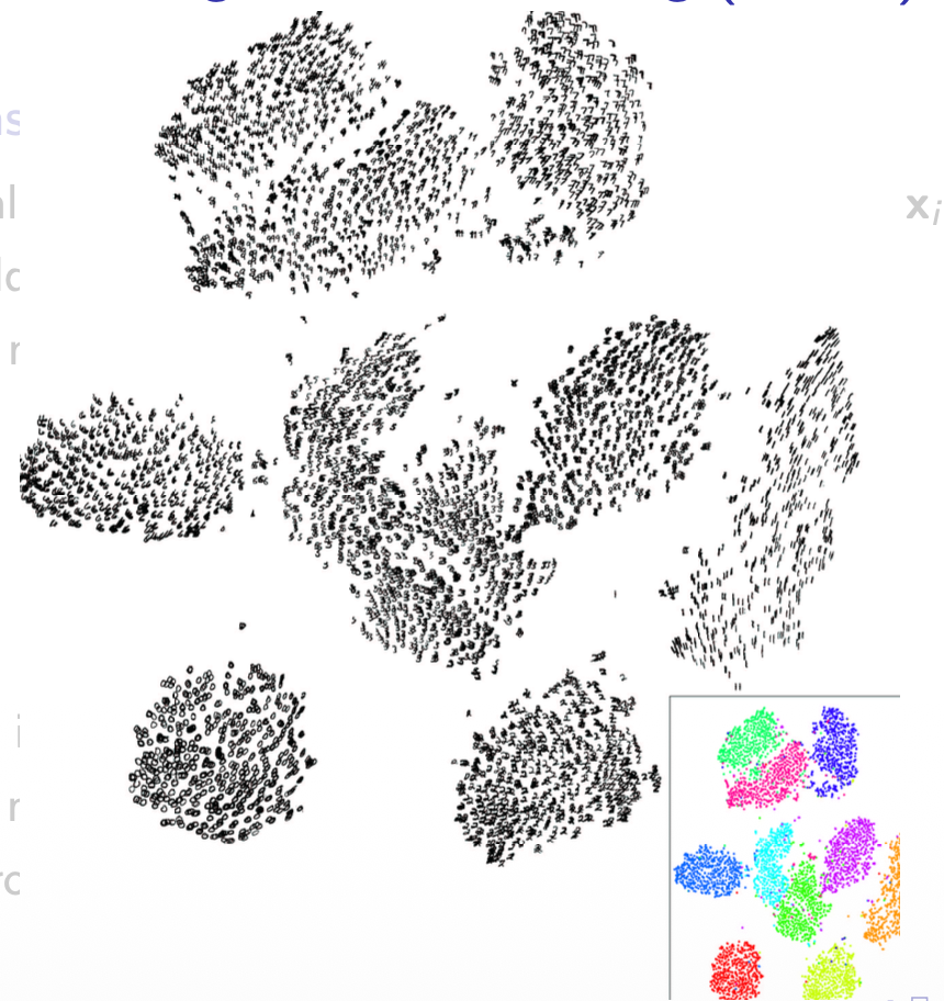
Why the student-t distribution matters: In high-dimensional space, the volume grows exponentially with distance, meaning many moderately distant points surround any given point. When projected down to 2D, there is insufficient area to place these points at appropriate distances without pushing them onto closer neighbors (the crowding problem).

Because the Student-t distribution has much heavier tails than a Gaussian:

• Moderately separated clusters in high dimensions can be pushed further apart in 2D while maintaining the same probability value qijqij​.
• It prevents the center of the embedding from collapsing into an uninterpretable ball, producing well-isolated cluster visual clusters (image above).

Uniform Manifold Approximation and Projection (U-MAP)

U-MAP

is a non-linear dimensionality reduction algorithm grounded in Riemannian geometry and algebraic topology. It models the data under the assumption that it lies on a low-dimensional manifold embedded in high-dimensional space, locally scaled so the data distribution appears roughly uniform.

• ML manifold $\approx$ smooth, low-dimensional subset of high-D space.
• Riemannian manifold = same thing with geometry (lengths, curvature, geodesics) explicitly defined

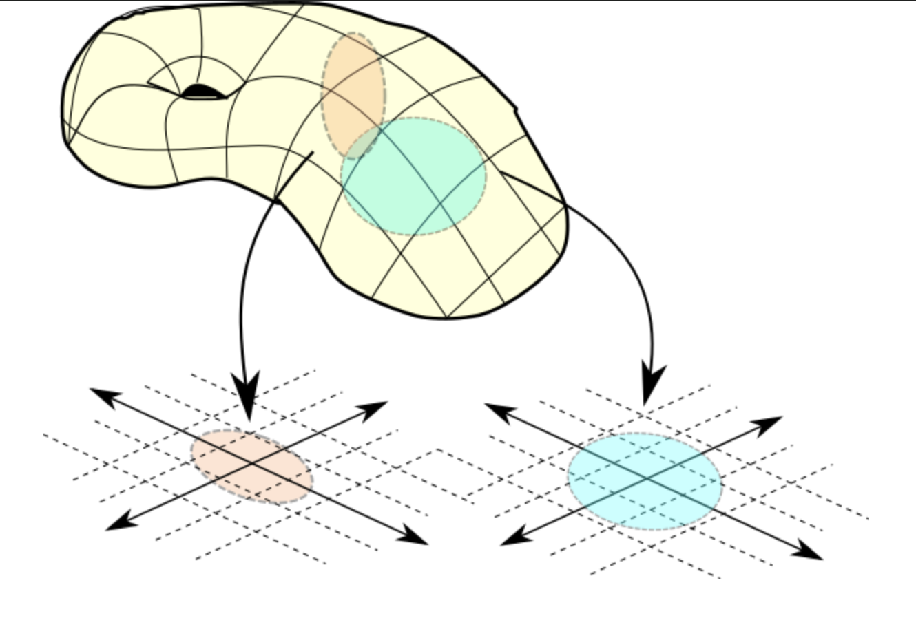
Core idea: Find a high-dimensionality manifold on which the data has uniform distribution

1. Weights are normalized by

• subtracting distance to nearest neighbor ${\rho }_i$
• scaling by ${\sigma }_i$: set so that ${\sum }_{K}w(x_i,x_j)=\text{constant}$

$$w({\mathbf{x}}_i,{\mathbf{x}}_j)=\exp \frac{-\max (0,d({\mathbf{x}}_i,{\mathbf{x}}_j))-{\rho }_i}{{\sigma }_i}$$

2. Iteratively optimise embeddings ${\mathbf{y}}_i$ embedded distances preserve weights

Compared to t-SNE

• Substantially faster
• Generally better preservation of global structure

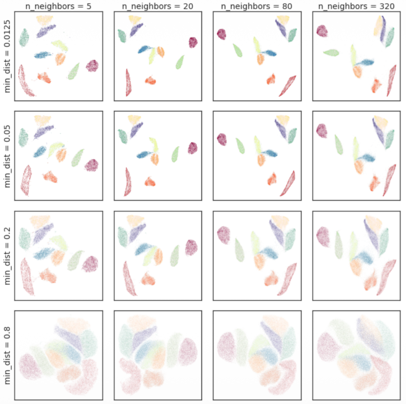
• n_neighbors: Controls the balance between local and global structure. Low values focus purely on fine-grained manifold patches, while higher values incorporate larger neighborhood contexts to capture overall geometry.
• min_dist: Dictates the minimum allowable distance between points in the 2D embedding, controlling whether points clump into tight, dense islands or remain smoothly dispersed.