Kernel Trick

Motivation: Nonlinear decision boundaries

Linear methods fail when the true boundary is curved (e.g. a circle, or XOR). Lift the data into higher-dimensional space where it becomes linearly separable.

Key Idea

Transform $x\to \varphi (x)$ to a higher dimensional space.

$$\varphi :x\to \varphi (x),R^d\to F$$

Input space: the space where the points $x_i$ are located Feature space: the space of $\varphi (x_i)$ after transformation

Linear operation in the feature space is equivalent to non-linear operation in the input space

XOR

The map $\varphi (x_1,x_2,x_3,x_4)$ makes XOR separable: the product coordinate captures the interaction.

$x_1,x_2\to z_1,z_2,z_3$, where $z_1=\sqrt{2}{x}_1{x}_2$, $z_2=x_1^2$, $z_3=x_2^2$

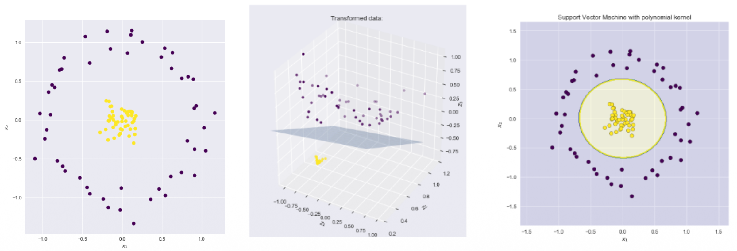
In the original 2D space $(x_1,x_2)$ on the left, the yellow and purple points form concentric circles. A standard SVM cannot draw a straight line to separate these two classes.

So we apply a feature map $\varphi (x)$ that maps the 2D coordinates into a 3D feature space $(z_1,z_2,z_3)$ using specific polynomial transformation. In this new 3D space shown in the middle, the data is now linearly separable. The SVM can easily insert a flat 2D plane to slice between the points.

When that flat 3D decision boundary is translated back to the original 2D space, it forms the perfect circular boundary seen in the right plot.

The kernel trick and Gram matrix

The kernel method lets linear algorithms (like SVM) to operate in very high (even infinite-dimensional) feature spaces without ever explicitly computing the feature map.

In the dual representation of SVMs, the solution is expressed using a Gram matrix.

• Instead of computing standard dot products $(G_{ij}=x_i\cdot x_j)$, the algorithm replaces them with a kernel function: $K(x_i,x_j)=\varphi (x_i)\cdot \varphi (x_j)$
• If the algorithm depends exclusively on this Gram matrix, we never have to compute or know the actual high-dimensional features of $\varphi$.

What's the kernel trick buying us?

Nonlinear decision boundaries at linear-algorithm prices: skip the explicit high-dimensional lift while getting its expressive power.

Another POV: kernel function, being an inner product, is really a similarity measure between the objects

Properties of a valid kernel

To use a shortcut function $k(x,y)$ as a kernel, it must be a symmetric function where matrices formed by any finite subset of points are positive semi-definite

$${\alpha }^{T}K\alpha \ge 0,\forall \alpha$$

Theorem

A function $k:x\times y\to R$ can be written as $k(x,y)=\varphi (x)\cdot \varphi (y)$ where $\varphi (x)$ is a feature map $x\to \varphi (x)\in F$ iff $k(x,y)$ satisfies the semi-definiteness property.

Symmetric: the order of the inputs does not matter. $K_{ij}=K_{ji}$

Positive semi-definite (PSD): a matrix $K$ is PSD if multiplying it by our test vector $\alpha$ and its transpose always results in a number $\ge 0$, no matter what number are in the $\alpha$ vector.

So all of this allows us to check if $k(x,y)$ is a proper kernel without needing to know the feature map, i.e. using only properties of $k(x,y)$ itself.

Common Kernels

• Linear: $K(x,y)=x^{\top }y$ (inner product)
• Polynomial: $K(x,y)=(1+x^{\top }y{)}^p$ (inner product, degree $p$ i.e. polynomial order)
• Gaussian: $K(x,y)=\exp (-\gamma ||x-y|{|}^2)$
• RBF (Radial Basis Function): $K(x,y)=\exp (-\frac{||x-y|{|}^2}{c})$
  • if $c$ is very small $\to$ the model considers all data to be dissimilar, which leads to over-fitting
  • if $c$ is very large $\to$ the model considers all data to be very similar, which leads to under-fitting.

Predicting a new point $x$: we don’t need $\varphi (x)$ explicitly. The model evaluates the sign of the decision function: $\hat{y}(x)=\mathrm{sign}\left({\sum }_i{\alpha }_i{y}_{i}k(x_i,x)+b\right)$

Each non-zero ${\alpha }_i$ indicates that corresponding $x_i$ is a support vector.

Complexity

• Linear-kernel SVM: $O(nd)$ training, $O(d)$ test time
• General-kernel SVM: $O(n^{2}d)$ to build the Gram matrix at training, $O(nd)$ test time (loop over support vectors)

So kernels aren’t free: there’s a dataset-size penalty. Worth it when $d$ is small or moderate and the true boundary is nonlinear.