Probabilistic Models

Parametric Models

Data types matter:

• Numeric — continuous (age, income) or discrete (counts)
  • Regression
• Categorical — a fixed set of labels (blood type, country)
  • Classification

We have two types of models:

1. Discriminative Models: learn a $p(C\mid x)$ directly.

• .e.g logistic regression: $p(C\mid x)=\sigma (x,w)$
• classification, segmentation, descriptors

2. Generative Models: learn the joint distribution of the data and target, and use Bayes’ rule

• Bayes’ Rule: $\underset{\text{Posterior}}{\underbrace{p(\mathcal{C}\mid \mathbf{x})}}=\frac{\stackrel{\text{Likelihood}}{\overbrace{p(\mathbf{x}\mid \mathcal{C})}}\cdot \stackrel{\text{Prior}}{\overbrace{p(\mathcal{C})}}}{\underset{\text{Evidence}}{\underbrace{p(\mathbf{x})}}}$

Go through Bernoulli Distribution before the reading the rest.

What is the probability that you will have to wait exactly 5 minutes for your bus?

zero.

We cannot assign probabilities to values. Instead, we need to assign probabilities to value ranges. Here we reiterate the Probability Density Function.

Remember that PDF’s

• are non-negative everywhere, integrate to 1
• can be interpreted as relative probabilities, but not as probabilities.
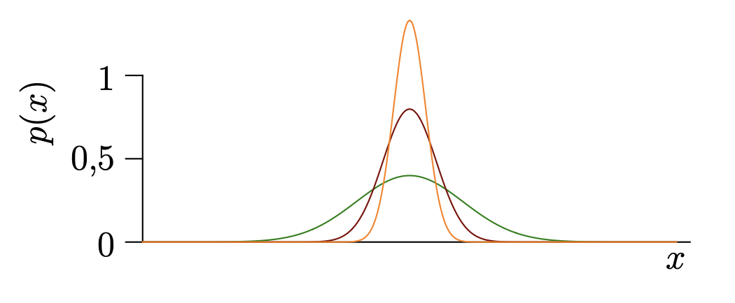
• can be larger than 1.

Something very interesting about the next example. The wider red distribution dominates the left extreme because its probability density function has higher variance. The narrow green distribution has a small variance, meaning its probability density drops to near zero very rapidly as you move away from its center. Because the green density decays so quickly on the far left, the wide, slowly decaying tail of the red distribution mathematically overtakes it, making the red class more probable at that extreme.

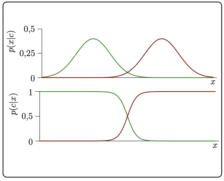
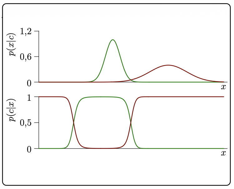
Mathematically, the distribution with the larger variance will always decay slower and eventually dominate at both limits

Central Limit Theorem

The sum of a sufficiently large number of independent, identically distributed (i.i.d.) variables with finite variance will have an approximately Gaussian distribution.

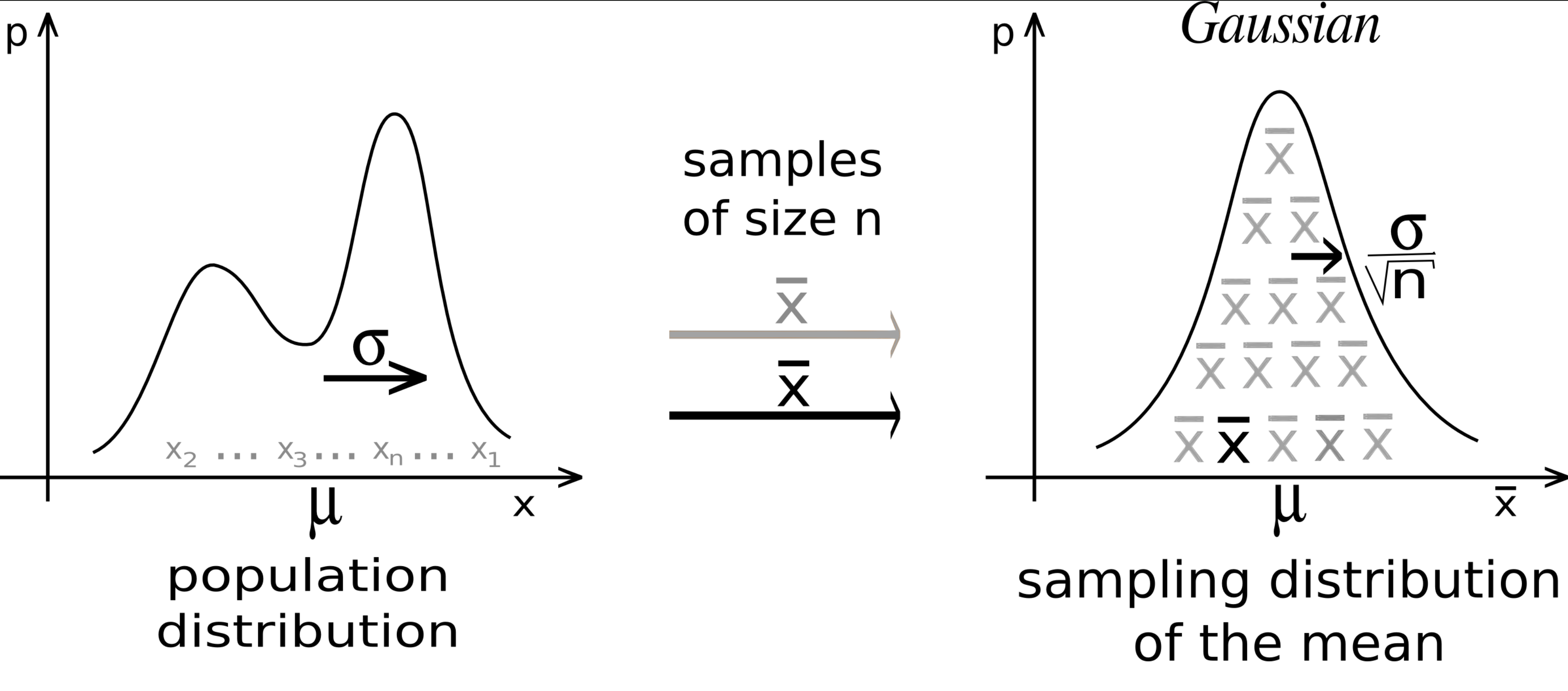
So in other words: take any distribution and randomly sample from it. Say if you sample at least 30 times, and you take the sum of those sampled values. Then repeat that process like 1000 times. If you plot the sums of those samples, it will follow a Normal Distribution.

Non-Parametric Models

Histogram Density Estimation

Instead of assuming a single functional representation of the distribution, we can use the training data itself. If we try to evaluate the distribution of data without assuming a parametric form of the density, we can use histograms.

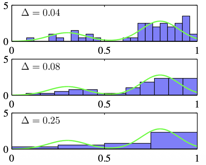
Disadvantages include:

• The bin positions and widths $△$ affect the density estimate
• The number of bins grows exponentially with the number of dimensions of the data

Kernel Density Estimation

For this reason we introduce Parzen Estimators — a technique that scales better with dimensionality.

• Consider a kernel function centered on each training data point ${\mathbf{x}}_n$
  • A common choice is the Gaussian where $h$ is the standard deviation of our Gaussian components and controls the smoothness of our estimate

$$p(\mathbf{x})=\frac{1}{N}\sum _{n=1}^N\frac{1}{(2\pi h^2{)}^{1/2}}\exp \left(-\frac{\Vert \mathbf{x}-{\mathbf{x}}_n{\Vert }^2}{2h^2}\right)$$ $$\stackrel{\begin{array}{c}\text{Probability density at}\\ \text{any location }\mathbf{x}\text{ in the space}\end{array}}{\overbrace{p(\mathbf{x})}}=\underset{\text{Normalise to sum to one}}{\underbrace{\frac{1}{N}}}\stackrel{\begin{array}{c}\text{Sum over all training}\\ \text{datapoints }{\mathbf{x}}_n\end{array}}{\overbrace{\sum _{n=1}^N}}\underset{\text{Kernel function, integrates to 1}}{\underbrace{\left[\frac{1}{(2\pi h^2{)}^{1/2}}\exp \left(-\frac{\Vert \mathbf{x}-{\mathbf{x}}_n{\Vert }^2}{2h^2}\right)\right]}}$$

• If this kernel is non-negative for all $\mathbf{x}$ and normalised, this gives a valid estimate of the data density.

Both methods require a hyperparameter to control the smoothness of the resulting density estimate. In histograms, this is the bin width $△$. In Gaussian Parzen estimators, this is the kernel’s standard deviation $h$. The final image demonstrates how sensitive the Parzen estimator is to this value

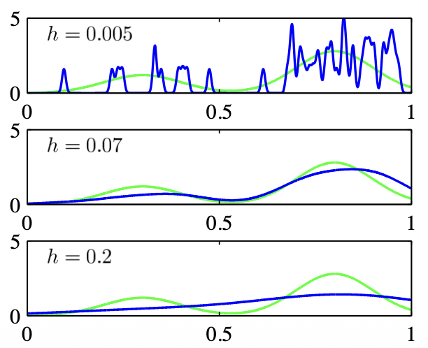
• A very small standard deviation ($h=0.005$) produces an extremely jagged, spiky distribution that overfits to individual data points.
• A very large standard deviation ($h=0.2$) produces an overly smooth, flat distribution that fails to capture the local peaks of the true underlying function.
• An intermediate value ($h=0.07$) provides a balanced density estimate that closely aligns with the actual underlying distribution.

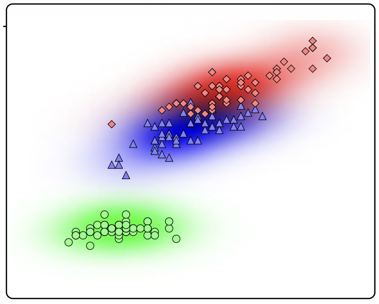
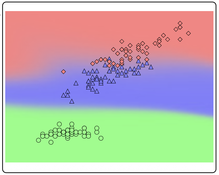
• the left image visualizes the joint probabilities, calculated as $p(x,c)=p(x\mid c)p(c)$ for three classes. The glowing regions represent the kernel density estimates build directly around the training data.
• the right image applies Bayes’ Theorem to those kernel estimates to compute the posterior probability, $p(c\mid x)$ for each class at any given location. These hard boundaries represent the decision regions a classifier would use to categorize a new, unseen data point into the red, blue, or green class based on its coordinates.

For example, The Nadaraya-Watson Model applies the concept of kernel density estimation to solve continuous regression problems, allowing us to predict a target variable $t$ based on an input $\mathbf{x}$.

Dual Representation

Many standard linear, parametric models can be mathematically rewritten so that instead of evaluating individual features directly, they evaluate pairs of training data points using a kernel function $k(\mathbf{x},{\mathbf{x}}^{\prime })$.

We often apply a fixed mapping $\varphi (\mathbf{x})$ to transform input data $\mathbf{x}$ into a new, higher-dimensional feature space to make it easier to classify or analyze. For models based on this mapping, the kernel function is defined mathematically as the scalar (dot) product of two transformed data points:

$$k(\mathbf{x},{\mathbf{x}}^{\prime })=\varphi (\mathbf{x}{)}^{\top }\varphi ({\mathbf{x}}^{\prime })$$

Also known as Kernel Substitution or Kernel Trick: allows an algorithm to implicitly compute the relationship between data points in a massive, high-dimensional space without ever actually having to calculate the expensive $\varphi (\mathbf{x})$ transformations explicitly.

• Because if an algorithm is structured so that the input vector $\mathbf{x}$ only ever appears inside scalar products, you can simply replace that standard product with a different kernel function.

Expectation

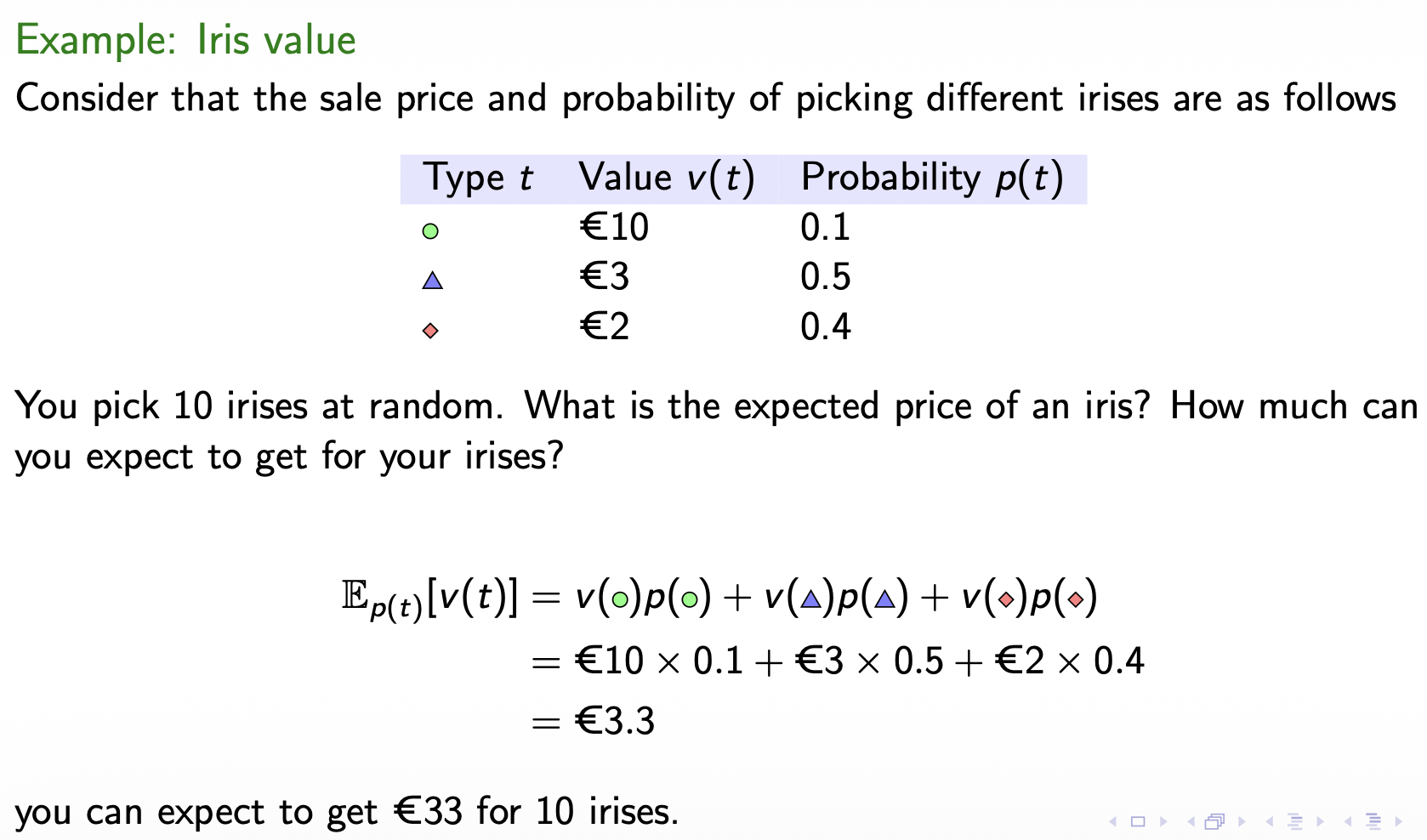
The expectation of a variable (or function of that variable) is the value that the long-term average of the function converges to, as the variable $x$ is distributed according to $p(x)$.

$${\mathbb{E}}_{p(x)}[f(x)]=\int f(x)p(x)dx$$

The objective is to minimize the probability of making a mistake. As shown in the Figure below, the total probability of a mistake is the sum of two scenarios: classifying a point as $C_2$ when it actually belongs to $C_1$ and vice-versa. Mathematically, this is expressed as integrals over the chosen decision regions:

$$p(\text{mistake})={\int }_{{\mathcal{R}}_1}p(\mathbf{x},{\mathcal{C}}_2)\mathrm{d}\mathbf{x}+{\int }_{{\mathcal{R}}_2}p(\mathbf{x},{\mathcal{C}}_1)\mathrm{d}\mathbf{x}$$

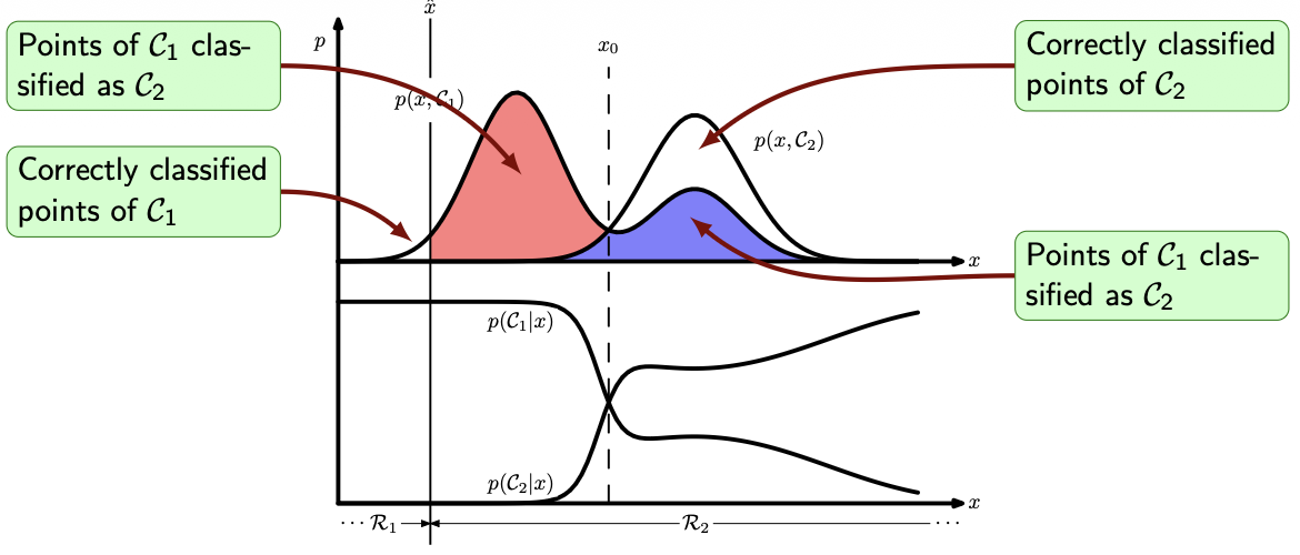
A decision boundary at an arbitrary point $\hat{\mathbf{x}}$ divides the space into region $R_1$​ (everything to the left) and region $R_2$​(everything to the right).

If we move the boundary $\hat{\mathbf{x}}$ to the optimal intersection point ${\mathbf{x}}_0$, the total shaded area (representing total errors) shrinks significantly. The red area disappears, leaving only a green region and a smaller blue region representing the unavoidable minimum overlap.

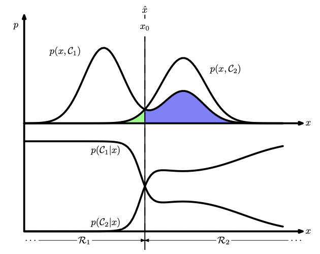
To minimize the total area of these mistakes, we must ensure that every single data point $\mathbf{x}$ is assigned to whichever class has the highest joint probability $p(\mathbf{x},C_k)$ at that specific location. Because the marginal probability $p(x)$ is constant across all classes at that location, this is mathematically identical to assigning the point to the class with the largest posterior probability $p(C_k\mid \mathbf{x})$. Therefore, the optimal decision boundary ${\mathbf{x}}_0$ always occurs exactly where the posterior probability curves cross.

Before going further, read Fundamentals of parameter estimation - Part I.

Maximum Likelihood with Simplifying Assumptions

We often lack data to train a model well by MLE. A standard Gaussian classification model with $c$ classes in $d$ dimensions requires calculating $c{d}^2$ parameters just for the covariance matrices, which naturally produces a complex, curved decision boundary.

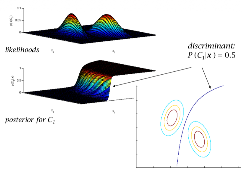
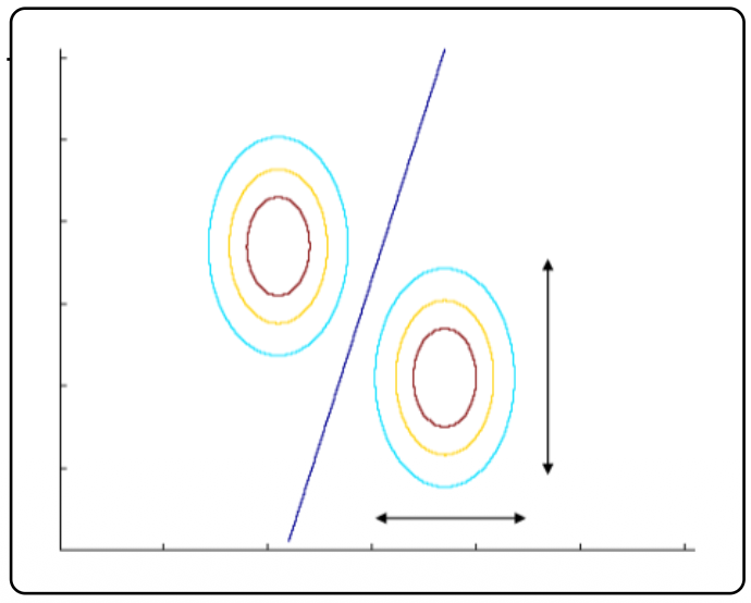
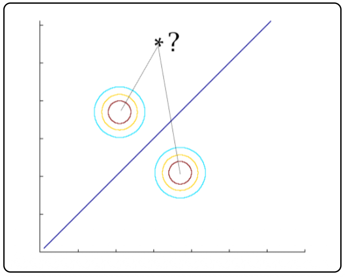
To reduce the number of parameters without losing too much discriminating power, we can apply three levels of simplifying assumptions:

1. Shared Covariance: Assuming all classes share the identical covariance matrix (${\Sigma }_1={\Sigma }_2$​) reduces the parameter count to $d^2$. Because the distributions now have the exact same shape and orientation, the complex curve straightens into a linear decision boundary.

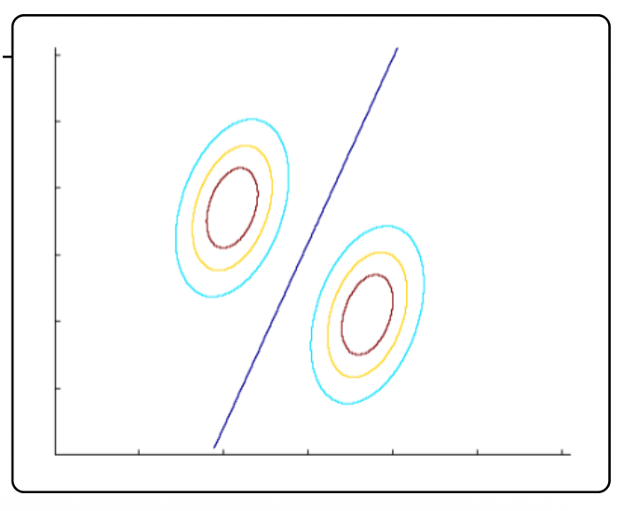
2. Diagonal Covariance: Assuming the covariance matrices are diagonal (${\Sigma }_1\leftarrow \text{diag}({\Sigma }_1$)) means treating all input dimensions as statistically independent. This reduces the required parameters down to $cd$. Visually, the contour ellipses are forced to align strictly with the coordinate axes

3. Spherical Covariance: The most extreme simplification assumes the covariance is a simple scalar multiple of the identity matrix (${\Sigma }_1=\sigma I$). This reduces the parameter count to just $c$. The distributions become perfect circles, meaning the classifier effectively just measures the straight-line distance from a new data point to each class center to make a decision.

Naive Bayes: Because it only computes 1D probabilities and multiplies them, it scales linearly with the number of features, making it computationally fast. It performs surprisingly well in real-world practice, but if the features are actually highly correlated, the model will output overly confident probability scores.

• conditional independence does not equal marginal independence!

$$p(x_1,\dots ,x_n)=\sum _{\mathcal{C}}p(x_1\mid \mathcal{C})\cdots p(x_N\mid \mathcal{C})p(\mathcal{C})\ne p(x_1)\cdots p(x_N)$$

Maximum A Posteriori (MAP) Learning

Earlier, MLE found the parameters that maximized the likelihood of the data. MAP learning flips this: it uses Bayes’ rule to find the most likely parameters ($\theta$), given the observed data ($\mathbf{x}$).

The denominator in Bayes’ rule requires integrating over all possible parameter values, which is often mathematically impossible (intractable) to compute. However, because the denominator is just a normalizing constant, we can completely ignore it when trying to find the maximum value. The optimal parameters are found simply by maximizing the product of the likelihood $p(\mathbf{x}\mid \theta )$ and the prior $p(\theta )$.

$$p(\mathbf{\theta }\mid \mathbf{x})=\frac{p(\mathbf{x}\mid \mathbf{\theta })p(\mathbf{\theta })}{\int p(\mathbf{x},\mathbf{\theta })\mathrm{d}\mathbf{\theta }}$$ $$\arg \underset{\theta }{\max }\frac{p(\mathbf{x}\mid \theta )p(\theta )}{\int p(\mathbf{x},\theta )\mathrm{d}\theta }=\arg \underset{\theta }{\max }p(\mathbf{x}\mid \theta )p(\theta )$$

• In the left image, with only a handful of data points, the glowing distribution is massive and diffuse, indicating that the model is highly uncertain about the true parameters.
• In the right image, as the sequence progresses and more data is collected, this posterior distribution rapidly shrinks and concentrates into a tiny, precise point exactly around the true parameter values.

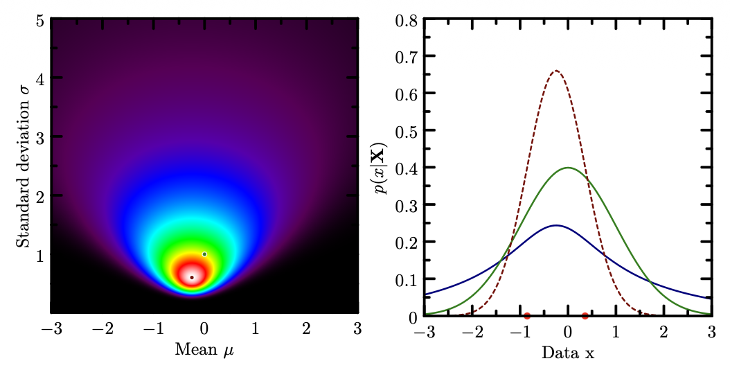
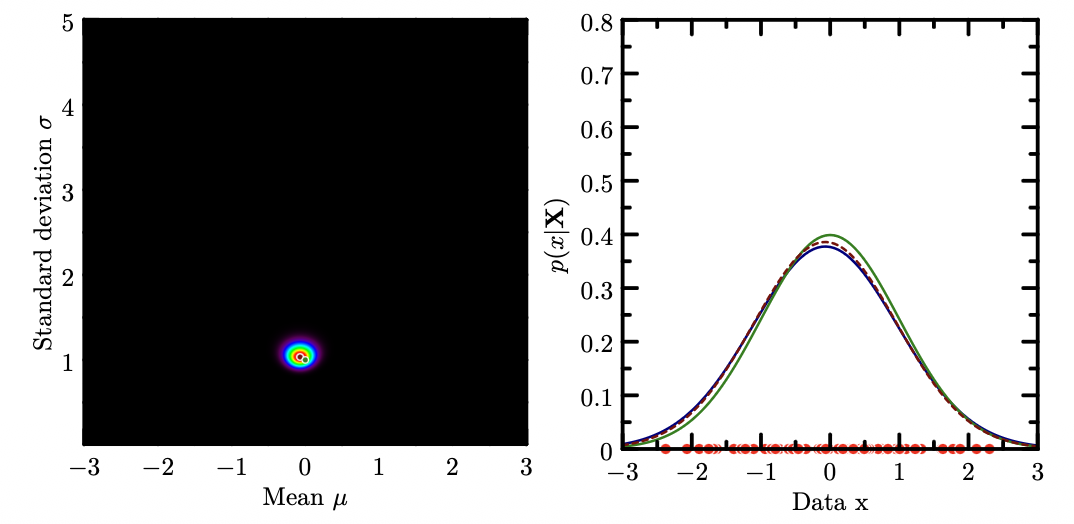
The primary takeaway is the behavior in the small-data regime. When data is extremely scarce, the standard point estimate (red dashed line) drastically overfits to those few points, outputting a peaked, overly confident distribution that misses the true green curve entirely. The Bayesian prediction (blue line) avoids this false confidence; it remains wide, flat, and cautious because it factors in the massive parameter uncertainty shown on the left. However, once you have abundant data, the parameter uncertainty vanishes, and the Bayesian curve, the point estimate, and the true distribution all safely converge into one.

page 89