Normalizing Flows

Resources: 1, 2, 3

Topic that I encountered in my GenAI Models and Robotic Applications course at Twente.

Basic Concept

Normalizing flows exploit the rule for change of variables. Normalizing flows begin with an initial distribution, and apply a sequence of K invertible transforms to formulate a new distribution.

Learns complex joint densities by decomposing the joint density into a product of one-dimensional conditional densities, where each $(x_i)$ depends on only the previous $(i-1)$ values (so just like in Markov Chains):

$$p_{model}(x)=\prod _{i}p\left(x_i|x_{1:i-1}\right)$$

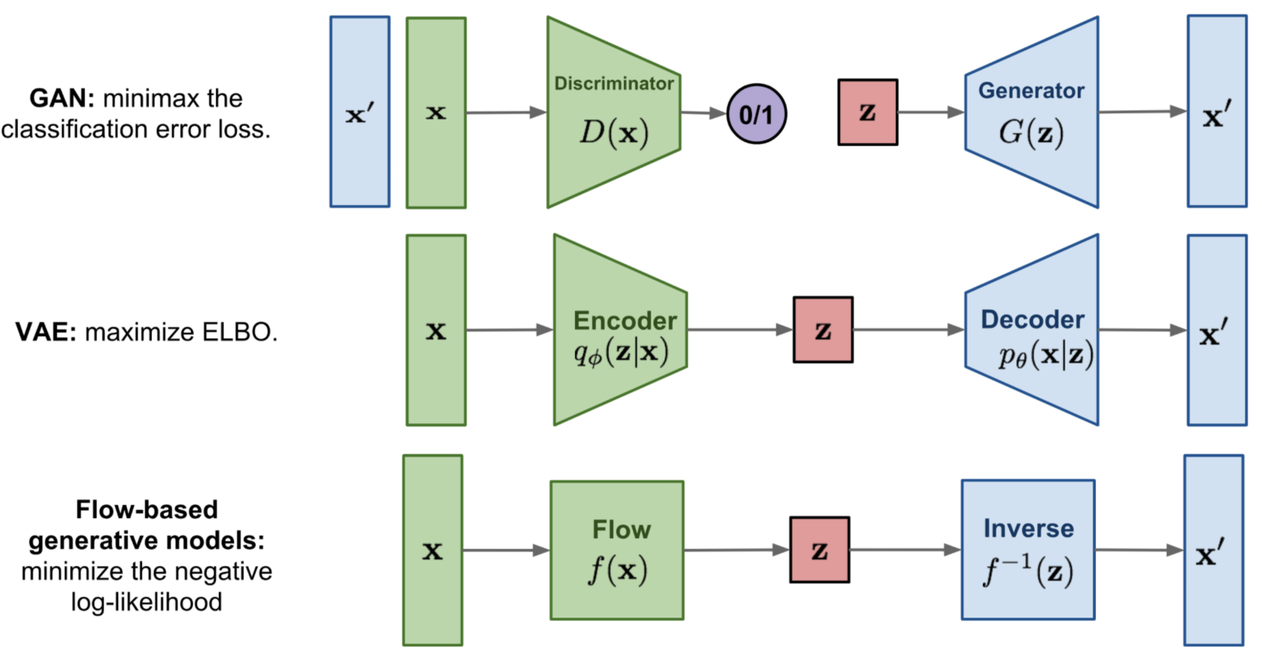
Quick summary of the difference between GAN, VAE, and flow-based generative models

1. Generative adversarial networks: GAN provides a smart solution to model the data generation, an unsupervised learning problem, as a supervised one. The discriminator model learns to distinguish the real data from the fake samples that are produced by the generator model. Two models are trained as they are playing a minimax game.
2. Variational autoencoders: VAE inexplicitly optimizes the log likelihood of the data by maximizing the evidence lower bound (ELBO). VAE is stochastic: it uses a stochastic encoder that samples $z$ from a learned distribution $q(z\mid x)$. It outputs a distribution. In VAEs, the model learns to approximate the mapping between data and latent Gaussian through separate encoder/decoder networks.
3. Flow-based generative models: A flow-based generative model is constructed by a sequence of invertible transformations. Unlike other two, the model explicitly learns the data distribution and therefore the loss function is simply the negative log likelihood. Normalizing Flows are deterministic: no randomness is added when transforming $x<->z$. It’s exact; we know what happens. In flows, the Gaussian is transformed through exact, invertible functions to match the data.

What are Normalizing Flows?

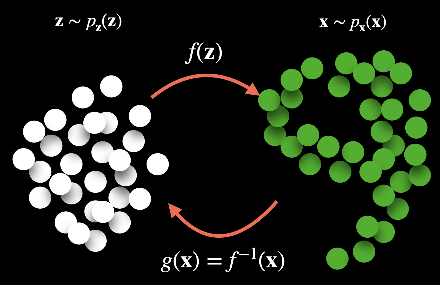
Normalizing flows learn an invertible transformation $f$ between data and latent variables: $x=f(z),z=f^{-1}(x)$

• $x$ is a target distribution data sample $\mathbf{x}\sim p_{\mathbf{x}}(\mathbf{x})$
• $z$ is a latent variable sampled from the source distribution $\mathbf{z}\sim p_{\mathbf{z}}(\mathbf{z})$

$$x=f(z)$$ $$p_x(x^{\prime })=p_z(z)\left|\det \left(\frac{\partial z}{\partial x}\right)\right|=p_z(z)\left|\det \left(\frac{\partial f^{-1}(x)}{\partial x}\right)\right|$$

If we define $J_f=\frac{\partial f^{-1}(x)}{\partial x}$, then we have:

$$p_x(x^{\prime })=p_z(z)\left|det[J_f]\right|$$

Intuitively, we can also write

$$p_z(z)=p_x(x^{\prime })\frac{1}{\left|det[J_f]\right|}=p_x(x^{\prime })\left|det[J_{f^{-1}}]\right|$$

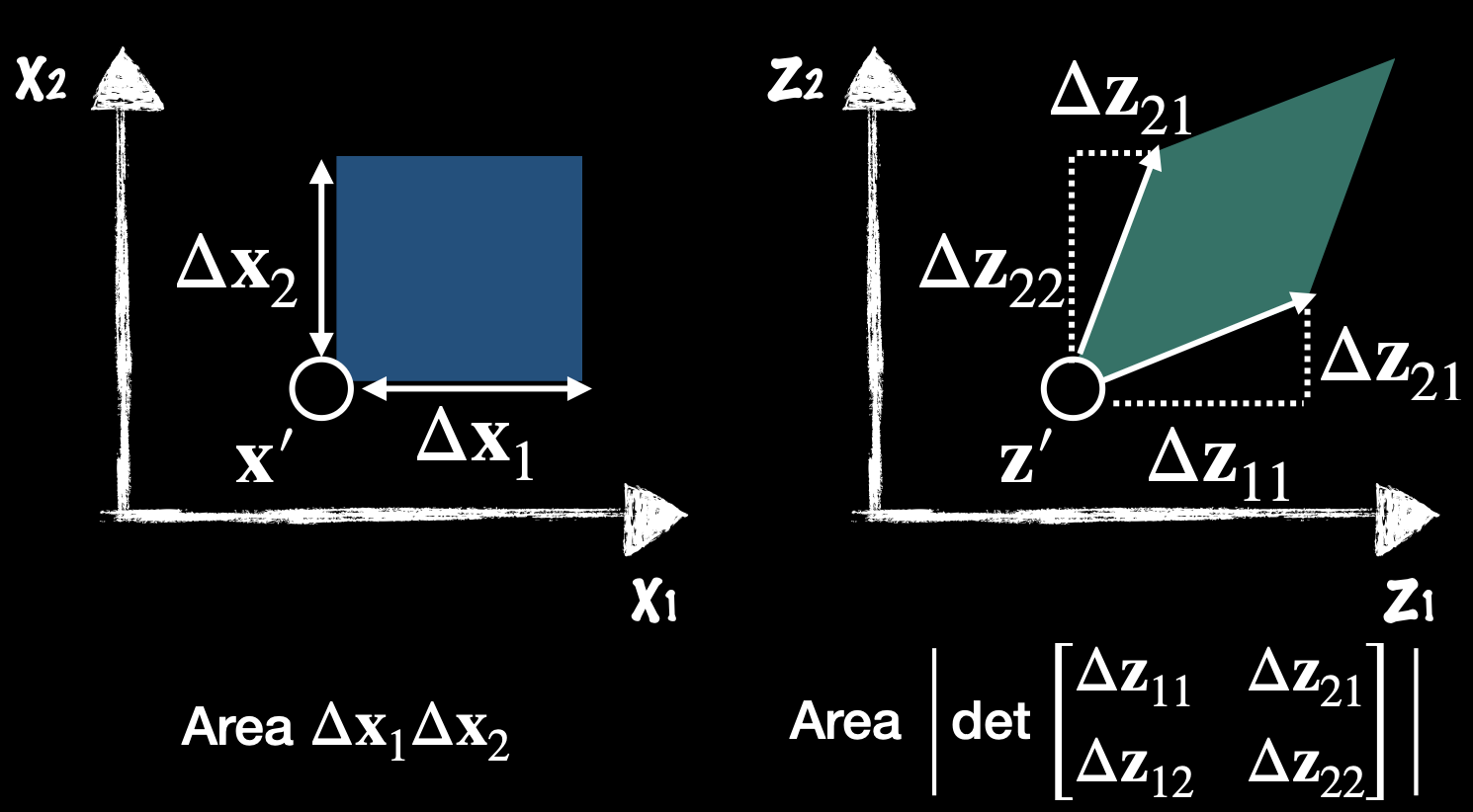
Explaining the Jacobian

$J_f$ is the Jacobian of the model from x to z (the inverse direction).

We can write in terms of probability density function (see Change-of-Variable Formula theorem)

Since $\mathbf{x}=f(\mathbf{z})$, we have:

$$J_f=\frac{\partial \mathbf{z}}{\partial \mathbf{x}}=\frac{\partial f^{-1}(\mathbf{x})}{\partial \mathbf{x}}$$

It describes how the transformation $f$ maps from the data space (x) to the latent space (z).

Conversely, $J_{f^{-1}}=\frac{\partial \mathbf{x}}{\partial \mathbf{z}}=\frac{\partial f}{\partial \mathbf{z}}$ maps from z to x.

$$\det [J_{f^{-1}}]=\frac{1}{\det [J_f]}$$

The restriction ($J\ne 0$) ensures invertibility, which is why normalizing flows require bijective transformations.

Here, $|\partial f^{-1}(x)|$ indicates the ratio between the area of rectangles defined in two different coordinate of variables  and  respectively

You can't just have $\mathbf{z}$

The function $f$ in normalizing flows is perfectly invertible. In normalizing flows, we care about density estimation, not reconstruction. The loss is based on the log likelihood of data $\mathbf{x}$ under the model (more below).

• That would basically be an Autoencoder.

• In training, data flows from $x\to z$ where $z=f^{-1}(x)$. We maximize $\log p_x(x^{\prime })$ (or minimize the negative log likelihood):

$$\log p_z(z)=\log p_x(x)+\log \left|det[J_{f^{-1}}]\right|$$ $$\log p_x(x)=\log p_z(z)+\log \left|det[J_f]\right|$$

• In sampling/generation, data flows from $z\to x$, sample $z\sim p(z)$ from the base distribution, and apply the forward flow: $x=f(z)$.

A normalizing flow transforms a simple distribution into a complex one by applying a sequence of invertible transformation functions. Flowing through a chain of transformations, we repeatedly substitute the variable for the new one according to the change of variables theorem and eventually obtain a probability distribution of the final target variable.

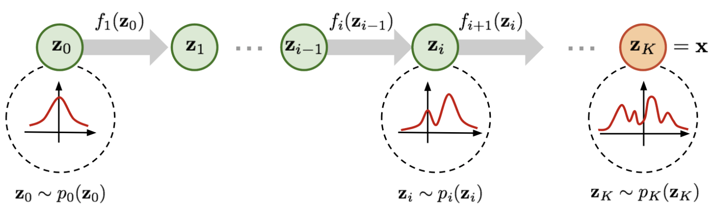
We apply a chain of invertible transformations (map the target distribution sequentially):

$$\mathbf{x}=f_K\circ f_{K-1}\circ ...\circ f_1(z)\text{, thus }\mathbf{z}=f^{-1}\circ ...\circ f_K^{-1}(\mathbf{x})$$

As defined in the figure above, we have

$$z_i\sim p_i(z_i)$$ $$z_i=f_i(z_{i-1}),\text{ thus }{z}_{i-1}=f_i^{-1}(z_i)$$

What does f look like? They’re generally Affine Transforms (affine coupling layer) since they are differentiable.

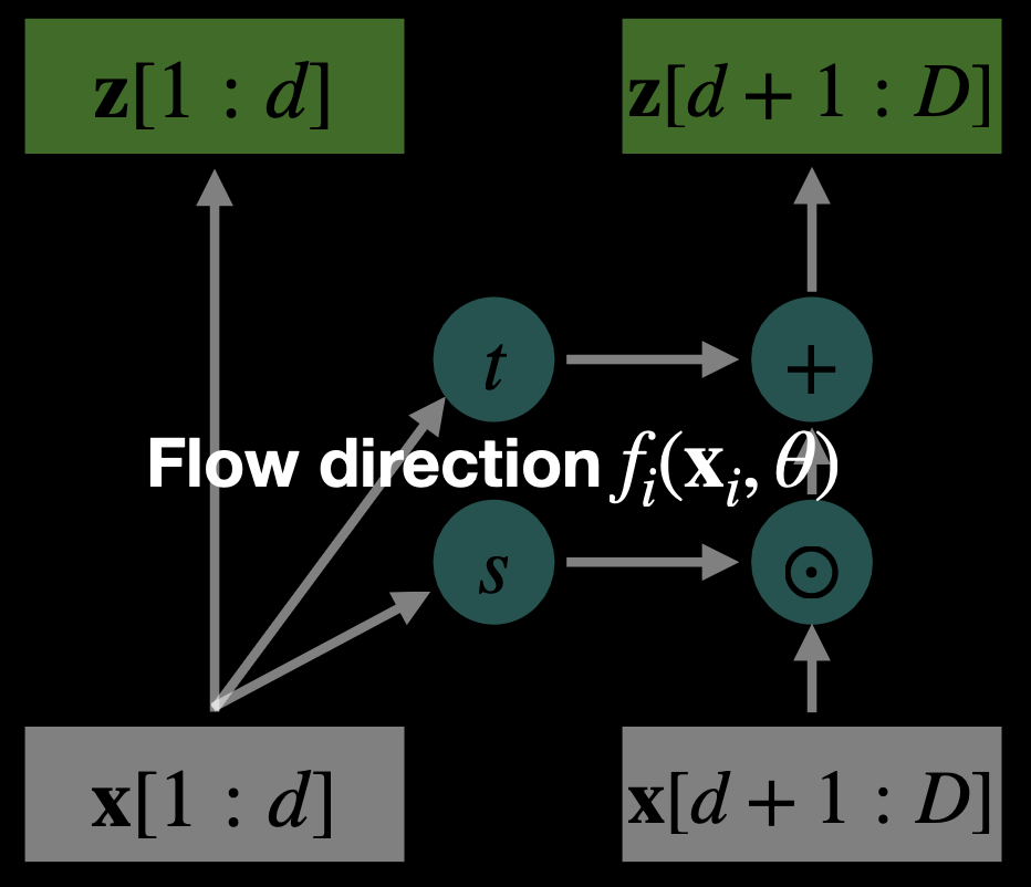
Flow Path (Forward Pass):

$$z[1:d]=x[1:d]$$ $$z[d+1:D]=x[d+1:D]\odot \exp (s_{\theta }(x[1:d]))+t_{\theta }(x[1:d])$$

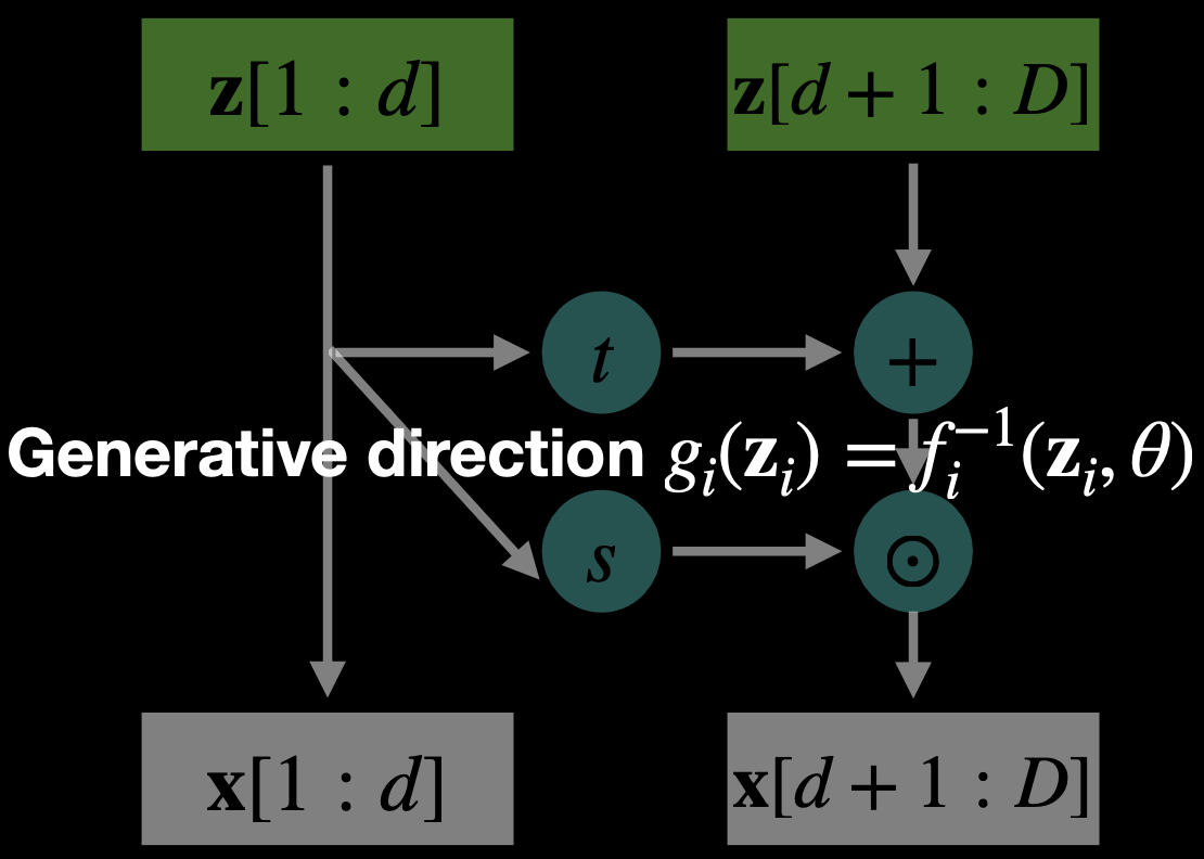
Generative Path (Inverse Pass):

$$x[1:d]=z[1:d]$$ $$x[d+1:D]=(z[d+1:D]-t_{\theta }(z[1:d]))\odot \exp (-s_{\theta }(z[1:d]))$$

• $s_{\theta }$ and $t_{\theta }$ are neural networks (often small CNNs or MLPs)
• Same parameters are reused in both directions.

How weight updates work in flow-based models

Training is done via maximum likelihood estimation (MLE) using the change-of-variables formula.

Change of Variables

Given $\mathbf{x}=f(z)$ and $\mathbf{z}\sim \mathcal{N}(0,I)$ (just a unit Gaussian):

$$\log p_x(x)=\log p_z(f^{-1}(x))+\log \left|\det \left(\frac{\partial f^{-1}}{\partial x}\right)\right|$$

We know that $\mathbf{z}=f^{-1}(\mathbf{x})$ and so we can write in the end:

$$\log p_z(z)=\log p_x(f(z))+\log \left|\det [J_{f^{-1}}]\right|$$

Training Steps

1. Inverse Pass: Given data $\mathbf{x}$, compute $\mathbf{z}=f^{-1}(\mathbf{x})$
2. Compute log-likelihood loss:

$$\mathcal{L}=-\log p_x(x)=-\log p_z(z)+\log \left|\det \left(\frac{\partial f}{\partial \mathbf{z}}\right)\right|$$

3. Backpropagate through:
   • the inverse transformations $f^{-1}$
   • the neural nets $s_{\theta }$ and $t_{\theta }$
   • the log-determinant term
4. Gradient Descent:
   • Use Adam/SGD to update parameters $\theta$ in $s_{\theta }$ and $t_{\theta }$