Lidar Odometry and Mapping in Real-time (LOAM)

Sources: paper, code repo.

This study is from 2014. I asked Gemini AI if it’s still highly relevant and the sectors it’s mostly applied in.

From Gemini AI

• LOAM is the go-to starting point for students and engineers. Because it is clean, lacks complex loop-closure logic, and uses standard libraries like Ceres Solver, it is the best way to learn how scan matching actually works without getting lost in “spaghetti code.”
• but its usage has shifted from being the “state-of-the-art” to being the foundational “Gold Standard” of the Lidar SLAM world
• Almost every modern Lidar SLAM algorithm used in self-driving cars or delivery robots today is a direct descendant of LOAM. It’s core concept remains the industry standard.

So the core concept would be:

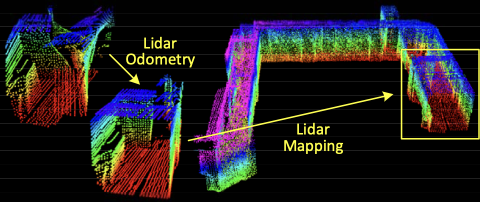
LOAM $\stackrel{\text{def}}{=}$ Splitting the problem into a high-frequency Odometry (fast) and a low-frequency Mapping (accurate)

SLAM typically seeks to optimize a large number of variables simultaneously.

• One algorithm performs odometry at a high frequency but low fidelity to estimate velocity of the lidar.
• Another algorithm runs at a frequency of an order of magnitude lower for fine matching and registration of the point cloud

The problem is hard because the range measurements are received at different times, and errors in motion estimation can cause mis-registration of the resulting point cloud. The method does not include loop closure.

• In the odometry algorithm, correspondences of the feature points are found by ensuring fast computation
• After which, mapping is conducted as batch optimization (similar to Iterative Closest Point (ICP)) to produce high-precision motion estimates and maps.

Sweep $\stackrel{\text{def}}{=}$ the lidar completes one time of scan coverage. They notate sweeps with $k\in Z^{+}$ and ${\mathcal{P}}_k$ to indicate the point cloud perceived during sweep $k$.

Lidar coordinate system {$L$} is a 3D coordinate system with its origin at the geometric center of the lidar. X-left, Y-upward, Z-forward. Coordinates of a point $i\in {\mathcal{P}}_k$ are denoted as $X_{(k,i)}^L$

World coordinate system {$W$} is a 3D coordinate system coinciding with {$L$} at the initial position. The coordinates of a point $i\in {\mathcal{P}}_k$ in {$W_k$} are $X_{(k,i)}^W$

Problem: Given a sequence of lidar cloud ${\mathcal{P}}_k$, $k\in Z^{+}$, compute the ego-motion of the lidar during each sweep $k$, and build a map with ${\mathcal{P}}_k$ for the traversed environment.

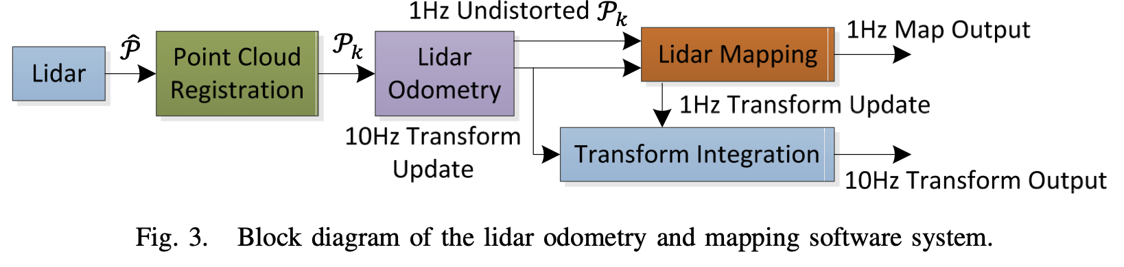
Lidar Odometry

• So the streamlined process sounds like this: During each sweep, the points received in a laser scan $\hat{\mathcal{P}}$ are registered in {$L$}. The combined point cloud during sweep $k$ forms ${\mathcal{P}}_k$ which is then processed in the two algorithms. The lidar odometry takes the point cloud and computes the motion of the lidar between two consecutive sweeps. The estimated motion is used to correct distortion in ${\mathcal{P}}_k$.
• 10[Hz] frequency

Lidar Mapping

• The outputs from Lidar Odometry are then processed, matching and registering the undistorted cloud onto a map at a frequency of 1[Hz]

Finally, the pose transforms published by the two algorithms are integrated to generate a transform output around 10[Hz], regarding the lidar pose with respect to the map.

Lidar Odometry

Feature Point Extraction

For a matching process the points that lie on sharp edges and planar surface patches are selected. The smoothness of a local surface is defined as:

$$c=\frac{1}{|S|\cdot \Vert X_{(k,i)}^L\Vert }\mid \mid \sum _{j\in S,j\ne i}\left(X_{(k,i)}^L-X_{(k,j)}^L\right)\mid \mid$$

• where $\mathcal{S}$ is the set of consecutive points $i$ in the same scan $k$.
• the code implementation is found at _scanRegistration.cpp, lines 305-315_.

The points in a scan are then sorted based on the c values:

• maximum $c$ values $\to$ edge points
• minimum $c$ values $\to$ planar points

To evenly distribute the feature points within the environment, they separate a scan into four identical subregions. Each subregion can provide maximally 2 edge points and 4 planar points

Which points do we discard, though?

The image kinda says it all. The point selection is implemented in the same file on lines 331-450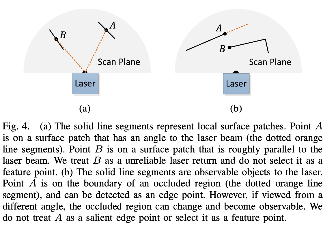

We want to avoid points whose surrounded points are selected, or points on local planar Scan Plane surfaces that are roughly parallel to the laser beams

• On the left side, it’s the latter case. If the laser beam is almost parallel to a surface (Point $B$), a tiny movement of the sensor will cause the laser to hit a completely different spot on that surface.
• On the right side, Point $A$ looks like an edge because it’s at the end of a visible line. However, it’s actually just where one object starts “blocking” (occluding) the view of whatever is behind it.

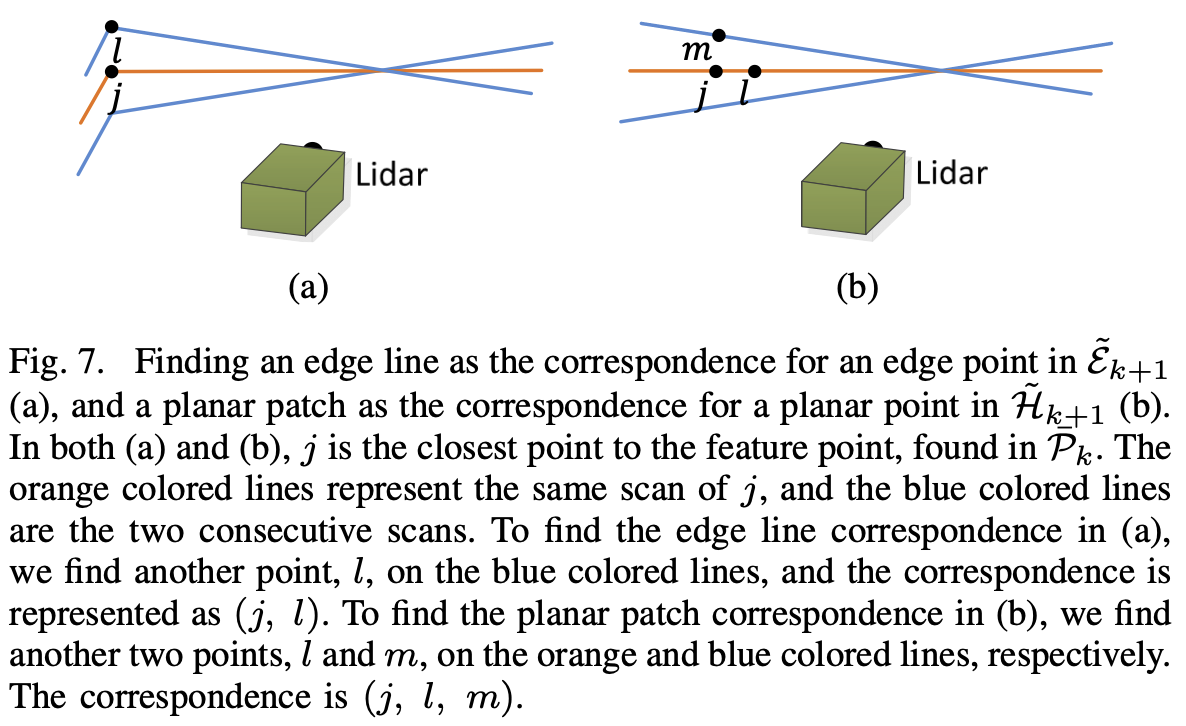
Feature Point Correspondence

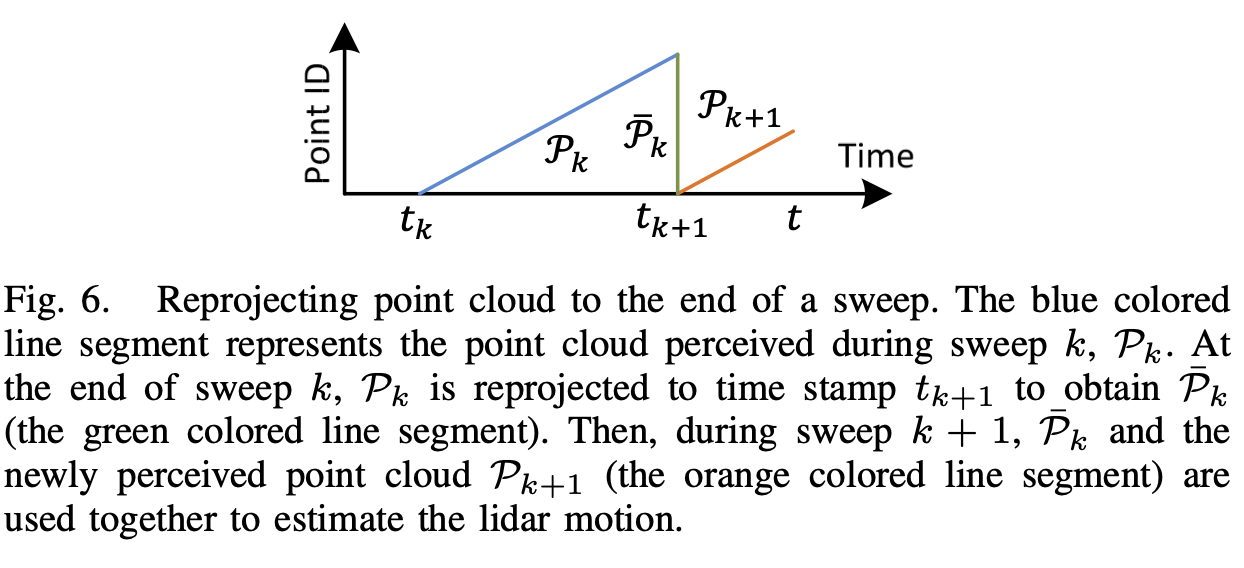
The algorithm estimates motion of the lidar within a sweep. Since the lidar is moving while it spins, the points at the start of the sweep ($t_k$​) and the end of the sweep ($t_{k+1}$) are skewed. As a solution, at the end of each sweep the point cloud ${\mathcal{P}}_k$ perceived at $t_k$ is reprojected at $t_{k+1}$ (i.e. $\bar{\mathcal{P}}$). During the next sweep $k+1$, $\bar{\mathcal{P}}$ is used together with the newly received point cloud, ${\mathcal{P}}_{k+1}$, to estimate the motion of the lidar. Again, the image says it all.

The corresponding code snippet can be found in laserOdometry.cpp on lines 325-524.

Let

• ${\mathcal{E}}_{k+1}$ be the set of edge points
• ${\mathcal{H}}_{k+1}$ be the set of planar points

We now want to find edge lines from ${\bar{\mathcal{P}}}_k$ as the correspondence between the two. The following Figure represents the procedure of finding an edge line as the correspondence of an edge point.

With the correspondences of the feature points found, now we can derive expressions to compute the distance from a feature point to its correspondence. Makes no sense to add them; they are hard to read so just return to the paper if needed.

Motion Estimation

They consider constant angular and linear velocities during a sweep $\to$ linear interpolations

They define the pose transform between [$t_{k+1},t$] as:

$$T_{k+1,i}^L=\frac{t_i-t_{k+1}}{t-t_{k+1}}{T}_{k+1}^L$$

Further, they establish a geometric relationship between ${\mathcal{E}}_{k+1}$ and ${\tilde{\mathcal{E}}}_{k+1}$ or ${\mathcal{H}}_{k+1}$ and ${\tilde{\mathcal{H}}}_{k+1}$.

$${\mathbf{X}}_{(k+1,i)}^L=\mathbf{R}{\tilde{\mathbf{X}}}_{(k+1,i)}^L+{\mathbf{T}}_{(k+1,i)}^L(1:3)$$

• $\mathbf{R}$ is Rodrigues Rotation Formula using lie algebra.

A geometric relationship between an edge or planar point and the distance to the corresponding edges or planar patches can be described as:

$$f_{\mathcal{E}}(X_{(k+1,i)}^L,T_{k+1}^L)=d_{\mathcal{E}},i\in {\mathcal{E}}_{k+1}$$ $$f_{\mathcal{H}}(X_{(k+1,i)}^L,T_{k+1}^L)=d_{\mathcal{H}},i\in {\mathcal{H}}_{k+1}$$

By stacking these two, we get a nonlinear function:

$$f(T_{k+1}^L)=d$$

This equation can be solved using Levenberg-Marquardt method by minimizing d to zero:

$$T_{k+1}^L\leftarrow T_{k+1}^L-(J^{T}J+\lambda \mathrm{diag}(J^{T}J){)}^{-1}{J}^{T}d$$

• where $J=\frac{\partial f}{\partial T_{k+1}^L}$. The calculation is performed in the laserOdometry.cpp file on lines 534-540.

Lidar Mapping

The mapping algorithm runs at a lower frequency then the odometry algorithm, and is called only once per sweep.

At the end of sweep $k+1$, the lidar odometry generates a undistorted point cloud ${\bar{\mathcal{P}}}_{k+1}$ and transform $T_{k+1}^L$. The mapping algorithm matches and registers ${\bar{\mathcal{P}}}_{k+1}$ in the world coordinates {$W$}.

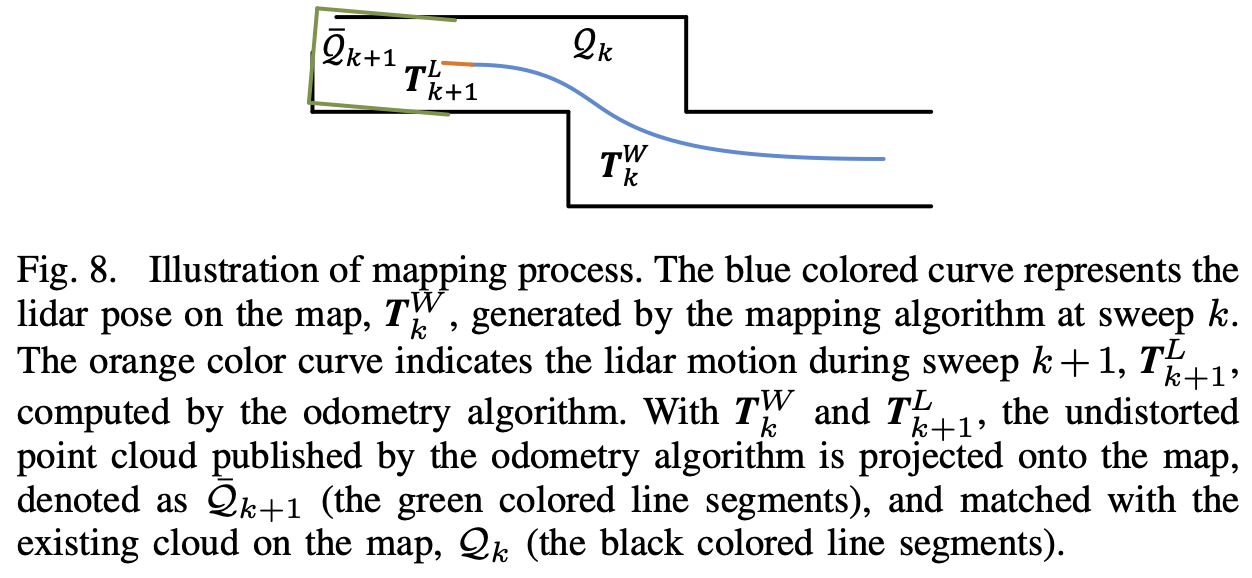
The corresponding code snippet can be found in laserMapping.cpp on lines 625-890

From here on they basically lost me with notations and details that are not important unless I want to understand the code implementation. This is the general idea of LOAM.