Neural ODEs

Source: paper

Instead of specifying a discrete sequence of hidden layers, we parameterize the derivative of the hidden state using a neural network.

These continuous-depth models have constant memory cost, adapt their evaluation strategy to each input, and can explicitly trade numerical precision for speed.

Related to Normalizing Flows, Transformers in depth and time.

Models such as residual networks and Normalizing Flows build complicated transformations by composing a sequence of transformations to a hidden state. They can be seen as an Euler discretization of a continuous transformation.

$${\mathbf{h}}_{t+1}={\mathbf{h}}_t+f({\mathbf{h}}_t,{\theta }_t)$$

A ODE network defines a vector field, which continuously transforms the state.

In this case we parametrize the continuous dynamics of hidden units using an ODE specified by a neural network.

$$\frac{d\mathbf{h}(t)}{dt}=f\left(\mathbf{h}(t),t,\theta \right)$$

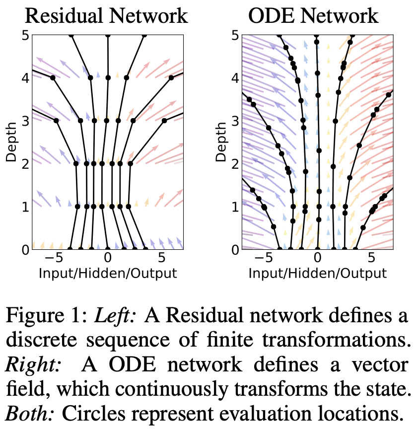
Starting from the input layer $\mathbf{h}(0)$, we can define the output layer $\mathbf{h}(T)$ to be the solution to this ODE initial value problem at some time $T$. This value can be computed by a black-box differential equation solver, which evaluates the hidden unit dynamics f wherever necessary to determine the solution with the desired accuracy.

Advantages

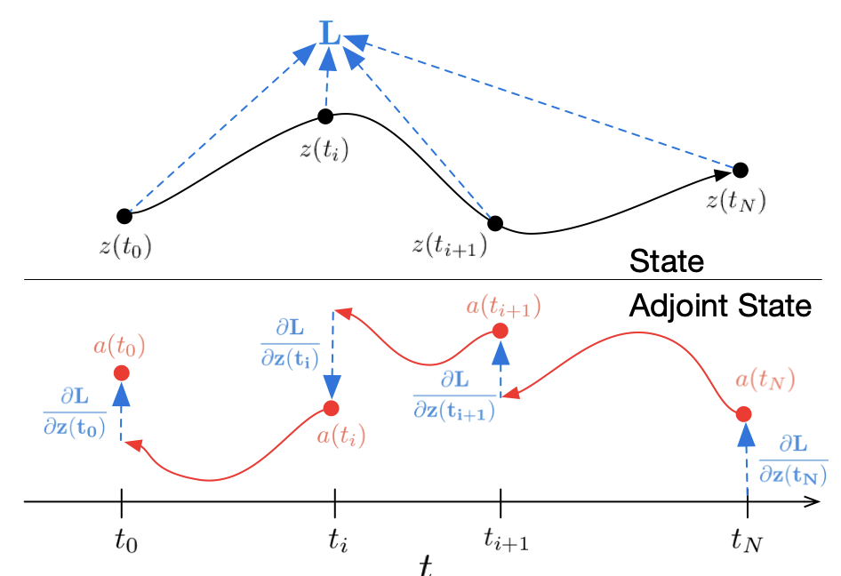
1. O(1) memory — instead of storing every layer’s activations for backprop, they use the adjoint sensitivity method: solve a second ODE backwards in time to get gradients, without ever storing the forward trajectory
2. Adaptive compute — modern ODE solvers (Runge-Kutta, etc.) pick their own step sizes to hit an error tolerance. So the network “depth” adapts per input automatically.
3. Continuous Normalizing Flows — for generative models, computing the log-det-Jacobian (needed for change-of-variables) is normally O($D^3$). In the continuous limit it becomes just a trace of the Jacobian, which is O(D) and doesn’t require restricting model architecture.

So the first bulletpoint is actually their main contribution. Differentiating through the operations of the forward pass is straightforward, but incurs a high memory cost and introduces additional numerical error. This approach scales linearly with problem size, has low memory cost, and explicitly controls numerical error.

To optimize the process, they first determine how the gradient of the loss depends on the hidden state $\mathbf{h}(t)$ at each instant i.e. the adjoint $\mathbf{a}(t)=\frac{\partial L}{\partial \mathbf{h}(t)}$:

$$\frac{d\mathbf{a}(t)}{dt}=-\mathbf{a}(t{)}^{\top }\frac{\partial f}{\partial \mathbf{h}}$$

• just solve this backwards from $t_1$ to $t_0$ and you get gradients w.r.t. the initial state, parameters $\theta$, and even integration times $t_0,t_1$ — all in one backward ODE solve.

For flows, just go with the trace idea mentioned earlier.