A practical on ML basics

to refresh some knowledge.

Geometry

1. Given the two points $(4,1)$ and $(-2,3)$, give an equation for the line through these two points. The equation should have the form:

$$w_0+w_1{x}_1+w_2{x}_2=0$$

There’s the line equation given by two points:

$$\frac{x-x_A}{x_B-x_A}=\frac{y-y_A}{y_B-y_A}$$

so after I plug in the values, I get:

$$\begin{array}{rl}\frac{x-4}{-2-4}& =\frac{y-1}{3-1}\\ 2x-8& =-6y+6\\ x+3y-7& =0\end{array}$$

If we substitute, the solution would be $w=\left(\begin{array}{c}{w}_0\\ w_1\\ w_2\end{array}\right)=\left(\begin{array}{c}-7\\ 1\\ 3\end{array}\right)$

2. Make a plot of the line and the vector $(w_1,w_2)$. The direction of $(w_1,w_2)$ is called the positive side of the line.

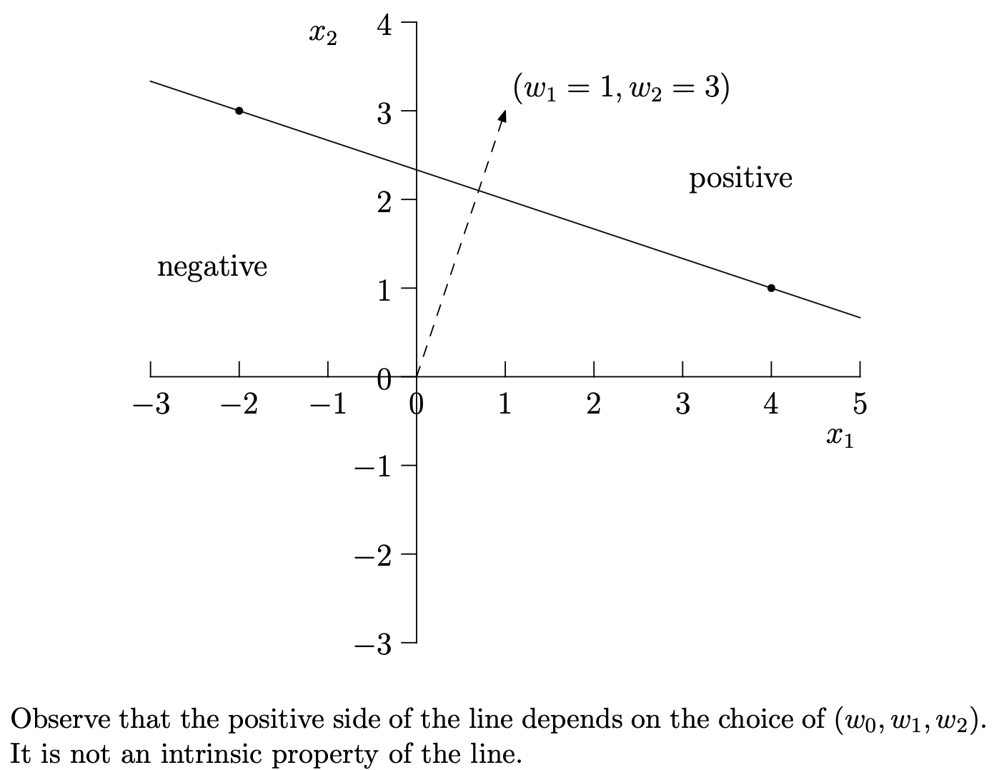
3. Consider the point $(x_1,x_2)=(4,3)$. Is this point on the positive side or negative side of the line? Also compute $w_0+w_1{x}_1+w_2{x}_2$ for this point.

I only need to plug the point into the line equation and see if it’s positive or negative.

$-7+4+9=6>0$ ⇒ on the positive side.

4. Show that the distance of the point $(x_1,x_2)=(4,3)$ to the line is equal to:

$$\frac{|w_0+w_{1}x1+w_2{x}_2|}{||(w_1,w_2)||}$$

The question is literally ask me to derive the formula, not simply use it. This is where I need to use vectors.

The concept is: move from the point along the normal direction until you hit the line; the distance moved is the answer.

What I know is that $(w_1{w}_2)$ is perpendicular to the line. Therefore, I need to make use of projections:

Let’s say that the point $(4,3)$ hits the line in point $y$ of coordinates $(y_1,y_2)$. A distance from a point to a line is the perpendicular from that point on the line. That means we have the same direction as $(w_1,w_2)=(1,3)$, since it’s also perpendicular on the line.

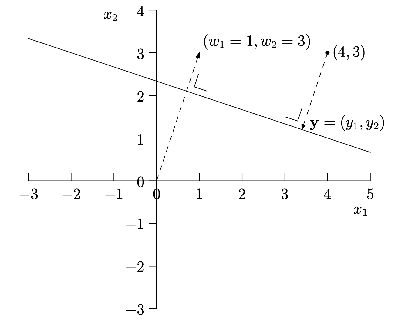
Since the point $y$ must lie on the line, we can compute $w+0+w_1{y}_1+w_2{y}_2=0$. Also, to go from $(4,3)$ straight to the line, I must move along the direction $(1,3)$. Any point along that direction, starting from $(4,3)$ can be written as:

start point + (scalar) $\times$ (direction) = $(4,3)+\lambda (1,3)$

λ is just “how far” I move along that direction — could be positive, negative, or zero.

$$\{\begin{array}{l}\left(\begin{array}{c}{y}_1\\ y_2\end{array}\right)=\left(\begin{array}{c}{x}_1\\ x_2\end{array}\right)+\lambda \left(\begin{array}{c}{w}_1\\ w_2\end{array}\right)\\ -7+y_1+3y_2=0\end{array}$$

Plug into the line equation:

$$\begin{array}{r}{w}_0+w_1(x_1+\lambda w_1)+w_2(x_2+\lambda w_2)=0\\ (w_0+w_1{x}_1+w_2{x}_2)+\lambda (w_1^2+w_2^2)=0\\ \lambda =\frac{-(w_0+w_1{x}_1+w_2{x}_2)}{||w_1,w_2|{|}^2}\end{array}$$

Since $y-(x_1,x_2)=\lambda (w_1,w_2)$, the distance between the point and $y$ is:

$$|\lambda |\cdot ||(w_1,w_2)||=\frac{|w_0+w_1{x}_1+w_2{x}_2|}{||w_1,w_2|{|}^2}\cdot ||w_1,w_2||=\frac{|w_0+w_1{x}_1+w_2{x}_2|}{||w_1,w_2||}$$

q.e.d.

5. What is the distance of the line to the origin $(0,0)$ and how can this be computed in terms of $(w_0,w_1,w_2)$?

I simply need to use the formula from the last question, and replace $(x_1,x_2)$ for $(0,0)$

$$\text{dist}=\frac{|w_0+w_{1}x1+w_2{x}_2|}{||(w_1,w_2)||}=\frac{|-7|}{\sqrt{1^2+3^2}}=\frac{7}{\sqrt{10}}$$

---

Calculus

1. Show that the derivative of $\sigma (y)=1/(1+e^{-y})$ w.r.t $y$ is given by:

$${\sigma }^{\prime }(y)=\sigma (y)(1-\sigma (y))$$

just know that $(e^u{)}^{\prime }=u^{\prime }\cdot e^u$

$$\begin{array}{rl}{\left(\begin{array}{c}\frac{1}{1+e^{-y}}\end{array}\right)}^{\prime }={\left(\begin{array}{c}\frac{f}{g}\end{array}\right)}^{\prime }& =\frac{f^{\prime }g-f{g}^{\prime }}{g^2}\\ & =\frac{e^{-y}}{(1+e^{-y}{)}^2}\\ & =\frac{1+e^{-y}-1}{(1+e^{-y}{)}^2}\\ & =\frac{1+e^{-y}}{(1+e^{-y}{)}^2}-\frac{1}{1+e^{-y}{)}^2}\\ & =\sigma (y)-\sigma (y{)}^2\\ & =\sigma (y)(1-\sigma (y)),q.e.d\end{array}$$

2. Show that:

• for $y$ large, i.e. $y\to \infty$, $\sigma (y)\approx 1$. I haven’t done limits since highschool. is this really ML?..

$$\underset{y\to \infty }{\lim }\frac{1}{1{+}_e^{-y}}=\frac{1}{1+0}=1$$

• for $y=0$, $\sigma (y)=0.5$

$$\underset{y\to 0}{\lim }\frac{1}{1{+}_e^{-y}}=\frac{1}{1+1}=0.5$$

• for $y$ small, i.e. $y\to -\infty$, $\sigma (y)\approx 0$

$$\underset{y\to -\infty }{\lim }\frac{1}{1{+}_e^{-y}}=\frac{1}{\infty }\to 0$$

• for $y$ large, ${\sigma }^{\prime }(y)\approx 0$

$$\underset{y\to \infty }{\lim }{\sigma }^{\prime }(y)=\underset{y\to \infty }{\lim }\sigma (y)(1-\sigma (y))=1(1-1)=0$$

3. From before, assume $w_0+w_{1}x1+w_2{x}_2=y$. Show that the partial derivative of $\sigma$ w.r.t $x_1$ is given by:

$$\frac{\partial \sigma }{\partial x_1}=\sigma (y)(1-\sigma (y))w_1$$

I already know ${\sigma }^{\prime }(y)=\sigma (y)(1-\sigma (y))$. And if I look at the line equation from above, $\frac{\partial \sigma }{\partial x_1}=w_1$. Therefore, we have the equation.

$$\frac{\partial \sigma }{\partial x_1}(y)={\sigma }^{\prime }(y)\frac{\partial y}{\partial x_1}(y)=\sigma (y)(1-\sigma (y))w_1$$

4. Once again assume that $w_0+w_{1}x1+w_2{x}_2=y$. Show that:

• the gradient of $\sigma$ w.r.t. the vector $w=(w_0,w_1,w_2)$ (denoted ${\nabla }_w\sigma (y))$ is given by ${\nabla }_w\sigma (y)=\sigma (y)(1-\sigma (y))x$, where $x$ is the vector $x=(1,x_1,x_2)$.

i see that each partial derivative corresponds to that vector: $\frac{\partial \sigma }{\partial w_0}=\sigma (y)(1-\sigma (y))\cdot 1$, $\frac{\partial \sigma }{\partial w_1}=\sigma (y)(1-\sigma (y))\cdot x_1$, $\frac{\partial \sigma }{\partial w_2}=\sigma (y)(1-\sigma (y))\cdot x_2$.

$${\nabla }_w\sigma (y)=\left(\begin{array}{c}\frac{\partial \sigma }{\partial w_0}(y),\frac{\partial \sigma }{\partial w_1}(y),\frac{\partial \sigma }{\partial w_2}(y)\end{array}\right)=\sigma (y)(1-\sigma (y))\cdot (1,x_1,x_2)=\sigma (y)(1-\sigma (y))\cdot x,q.e.d.$$

5. Show that:

• if $x_1$ is positive, then for $w_1\to \infty$ and other weights and input constant, $\frac{\partial \sigma }{\partial w_1}(y)\approx 0$

Since $w_0+w_{1}x1+w_2{x}_2=y$, with $w_0,w_2,x_1,x_2$ constants and $x_1>0$, as $w_1\to \infty$ we get $y\to \infty$.

I showed in the second subpoint that as $y\to \infty$, ${\sigma }^{\prime }(y)=\sigma (y)(1-\sigma (y))\approx 0$. The term from above would reduce to $\frac{\partial \sigma }{\partial w_1}(y)=\sigma (y)(1-\sigma (y))x_1$, where $x_1$ is a positive constant, which does not affect the end result of 0.

• if $x_1$ is negative, then for $w_1\to \infty$, $\frac{\partial \sigma }{\partial w_1}(y)\approx 0$

Since $w_0+w_{1}x1+w_2{x}_2=y$, with $w_0,w_2,x_1,x_2$ constants and $x_1<0$, as $w_1\to \infty$ we get $y\to -\infty$.

From part 2, as $y\to -\infty$, I showed that $\sigma (y)\approx 0$. So ${\sigma }^{\prime }(y)=\sigma (y)(1-\sigma (y))\approx 0(1-0)=0$.

Statistics and Probability theory

Consider $X=\{(1,4),(2,5),(-2,1),(-2,-3)\}$.

1. Compute the sample mean of $X$.

I would ASSUME it’s the overall mean over $x$ and $y$ axes: $(\frac{1+2-2-2}{4},\frac{4+5+1-3}{4})=(-0.25,1.75)$

2. Compute the covariance matrix of $X$.

Should be a $2\times 2$ matrix since we have two dimensions. We use the formula:

$$\sum =\frac{1}{N}\sum _i(x_i-\mu )(x_i-\mu {)}^{\top }$$

Apparently, this is the biased (maximum likelihood estimate) — on average it slightly underestimates the true variance, because I used the data itself to compute $\mu$. If they said something like “assume this is the full population”, or “maximum likelihood estimate of…”, then I use $N$.

Therefore, dividing by $N-1$ corrects that bias. Apparently this is the norm in libraries as well.

$$\sum =\frac{1}{N-1}\sum _i(x_i-\mu )(x_i-\mu {)}^{\top }$$

So the answer is:

$$\sum =\left(\begin{array}{c}4.256.5833\\ 6.573312.9167\end{array}\right)$$

3. Compute, based on the covariance matrix, the correlation between $x_1$ (the first component) and $x_2$.

Covariance tells me direction of the relationship but its size depends on the units/scale of $X_1$ and $X_2$ — so it’s not comparable across datasets. Correlation fixes this by standardizing.

correlation = "covariance after removing the scale"

Start with the covariance:

$$Cov(X_1,X_2)=E[(X_1-{\mu }_1)(X_2-{\mu }_2)]$$

This in itself mixes the units of $X_1$ and $X_2$ (e.g. $X_1$ is in meters, $X_2$ is in kg), then we would have a meter-kg meaningless scale. To remove the scale dependence, standardize each variable first — divide by its own deviation:

$$Z_1=\frac{X_1-{\mu }_1}{{\sigma }_1},Z_2=\frac{X_2-{\mu }_2}{{\sigma }_2}$$

Then the correlation is just the covariance of the standardized variables:

By definition, covaiance of any two variables is:

$$Cov(Z_1,Z_2)=E[(Z_1-E[Z_1])\cdot (Z_2-E[Z_2])]$$

But I standardized the data. $Z_1=\frac{X_1-{\mu }_1}{\sigma }$ has mean 0. Same for $Z_2$. So $E[Z_1]=E[Z_2]=0$.

$$\rho =Cov(Z_1,Z_2)=E[Z_1\cdot Z_2]=Cov(X_1,X_2)/({\sigma }_1\cdot {\sigma }_2)=\frac{Cov(X_1,X_2)}{\sqrt{{\sigma }_1\cdot {\sigma }_2}}=\frac{6.5833}{\sqrt{4.25\times 12.9167}}=0.8885$$

• remember that $\sum =\left[\begin{array}{c}\text{Var}(X_1),\text{Cov}(X_1,X_2)\\ \text{Cov}(X_1,X_2),\text{Var}(X_2)\end{array}\right]$. So get them directly from the previous point.

4. Compute the eigenvalues and eigenvectors of the covariance matrix of part b. What is the covariance matrix if we transform the data points into coordinates w.r.t these eigenvectors?

From ML Preliminaries, we call e an eigenvector and $\lambda$ the corresponding eigenvalue of matrix A if:

$$Ae=\lambda e$$

So we start with this formula:

$$\begin{array}{rl}Ae& =\lambda e\\ Ae-\lambda e& =0\\ (A-\lambda I)e& =0\end{array}$$

I want a nonzero eigenvector $e$. The equation from above has nonzero solutions only when the matrix $A-\lambda I$ is singular (non-invertible) — otherwise the solution would be $e=0$.

A matrix is singular exactly when its determinant is 0. Also called characteristic equation.

$$det(A-\lambda I)=0$$

So I use it for the covariance matrix $\sum$

$$\begin{array}{rl}det(\sum -\lambda I)& =0\\ det(\left(\begin{array}{c}4.256.5833\\ 6.573312.9167\end{array}\right)-\left(\begin{array}{c}\lambda 0\\ 0\lambda \end{array}\right))& =0\\ i.e.(4.25-\lambda )(12.9167-\lambda )-6.5833\cdot 6.5733& =0\\ {\lambda }^2-17.1667\lambda +11.5566& =0\\ \text{Solving is simply finding the solutions}(\Delta )& \\ {\lambda }_1\approx 16.4648,{\lambda }_2\approx 0.7018& \end{array}$$

Now for the eigenvectors, this gives a system of equations to solve for $e=(e_1,e_2)$. So from the formula above:

$$\sum -{\lambda }_{1}I=\left[\begin{array}{c}-12.2148,6.5833\\ 6.5833,-3.5481\end{array}\right]$$

So the equation $(\sum -\lambda I)e=0$ becomes:

$$\begin{array}{r}\{\begin{array}{ll}-12.2148\cdot e_1+6.8533\cdot e_2& =0\\ 6.5833\cdot e_1-3.5481\cdot e_2& =0\end{array}\end{array}$$

These two are just multiples of each other (that’s what “singular matrix” means — determinant 0), so I only need one of them. The first yields $e_2\approx 1.8555\cdot e_1$

Now I need to normalize. It’s convention so eigenvectors are comparable/unique:

$$|e|=\sqrt{1^2+1.8555^2}\approx 2.1078$$

So $e_1$ normalized would be:

$$e=(1/2.1078,1.8555/2.1078)\approx (0.4744,0.8804)$$

eigenvectors are only defined up to sign; both $e$ and $-e$ are equally valid since $-e$ is also a solution to the equation above.

Doing the same step for ${\lambda }_2\approx 0.7018$ yields $e_2\approx (0.8803,-0.4745)$.

One can see the eigenvectors have the same values inside, just swapped in position, with one sign flipped.

Eigenvectors of a symmetric matrix are orthogonal — perpendicular to each other. For a 2D vector, if I have a vector $(a,b)$, a perpendicular vector is always $(-b,a)$ or $(b,-a)$.

• Now the second part: what is the cov matrix if we transform the data points into coordinates w.r.t these eigenvectors?

I build a matrix $E$ whose columns are the eigenvectors:

$$E=\left[\begin{array}{c}0.4744,0.8803\\ 0.8804-0.4745\end{array}\right]$$

To express a data point $x$ (as a column vector, mean-centered) in the new coordinate system, project it onto each eigenvector using the dot product:

$$x^{\prime }=E^{\top }x$$

complete here…