Multi Layer Perceptron (MLP)

The topics introduced in Linear Regression with Gradient Descent suffer from one big drawback: linearity is assumed. However real-life data is mostly never linear and Representation Learning is a very efficient way of learning the underlying relationships of the data.

MLPs are basically Feedforward Neural Networks:

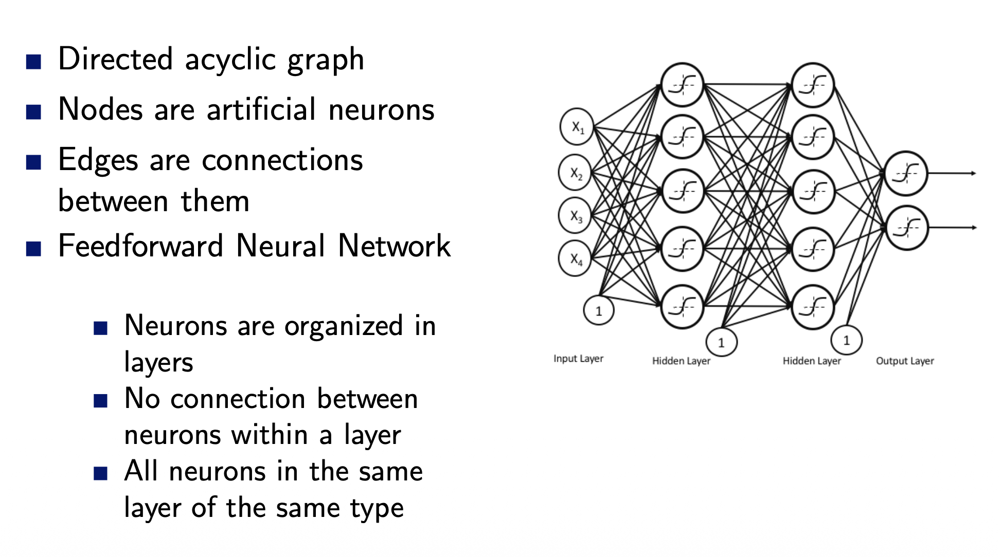
Each layer creates a new representation of the input data.

We can create computational graphs out of MLPs too once we consolidate them in blocks.

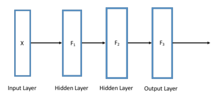
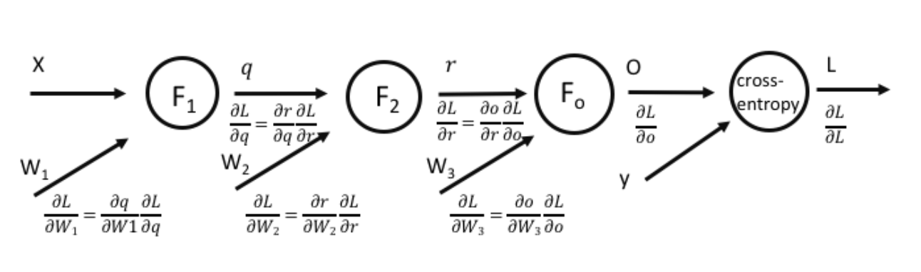
Small reminder that for classification, the $\text{softmax}$ function represents normalized probabilities that sum up to 1. (strictly positive)

Design decisions

• Output activation function — $\text{softmax}$
  • $p(y=j\mid x)=\frac{e^{{\mathbf{x}}^{\top }{w}_j}}{{\sum }_{k=1}^n{e}^{{\mathbf{x}}^{\top }{w}_k}}$
  • Multinoulli output distributions
• Hidden layer activation function — ReLU
• Architecture of the model
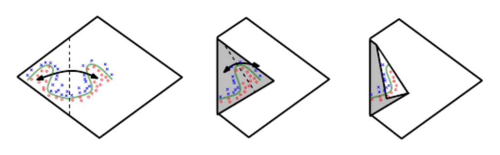
  • Number of hidden layers (e.g. 2) — deeper
    • The segments grow exponentially
  • Number of neurons/layer (e.g. 256) — wider
    • The segments grow polynomialy.
  • This refers to how a neural network divides the input space into different regions (or piecewise linear segments) to approximate a complex function.

• Loss function (e.g. Cross entropy)
  • Differentiable (smooth)
  • Monotonically increasing with the distance from the target value

In case we use $\text{sigmoid}$ instead of $\text{softmax}$, we get Bernoulli output distributions — $p(y=1\mid x)=\frac{1}{1+e^{-{\mathbf{w}}^{\top }\mathbf{x}}}$

If all neurons are linear, the MLP is linear, which limits the generalization! Additionally, capacity scales poorly — to learn a complex function the model needs exponentially more neurons.

Universal Approximation Theorem (Hornik, 1991)

A single hidden layer neural network with a linear output unit can approximate any continuous function arbitrarily well, given enough units.

Mind the two ideas above, however!

page 45