Linear Discriminants

See the easiest example: Two class classification

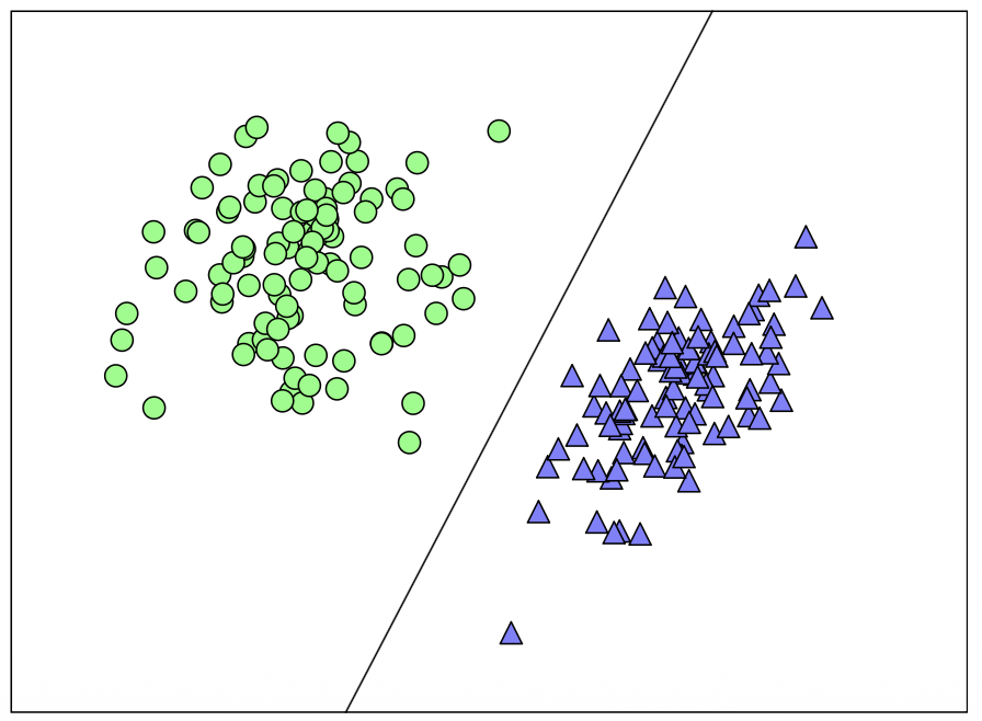
• Get class labels as a function of the features: $\{\begin{array}{l}{C}_0\text{, if y(x) > 0}\\ C_1\text{, if y(x) < 0}\end{array}$
• Discriminant: $y(x)=0$
• Linear classifier $\to$ $y(x)=0$ is a linear function of $x$.

$$y(x)=w_0+w^{\top }x$$

From a geometric view, the slope is determined by $w$, offset from origin by $w_o$ i.e. $\frac{w_0}{||w||}$.

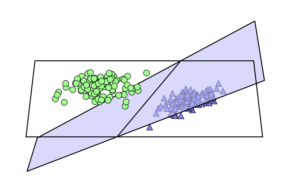
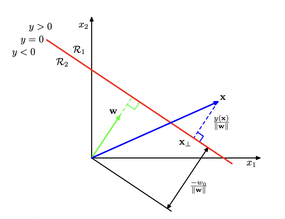
For convenience, fold the bias in $\tilde{w}=(w_0,w_1,\dots w_d)$ and ${\tilde{x}}^{\top }=(1,x_1,\dots x_D)$. So that $y(x)={\tilde{w}}^{\top }\tilde{x}$. The hyperplane equation becomes ${\tilde{w}}^{\top }\tilde{x}=0$. We use $w$ to denote $\tilde{w}$ from now on.

• Modify $x\to$ classify a new datapoint
• Modify $w\to$ change the discriminant

Choosing a good classifier

• Minimize misclassified training points
• Maximize separation of the most ambiguous points
• Maximize data probability

If we generalize to $K$ classes, simply combine multiple 2-class classifiers, and watch out for ambiguous regions. The result depends on the slope $|w_k|$, not just the decision itself.

• use $C=C_k<=>y_k(x)>y_j(x)\forall j\ne k\text{, where }{y}_k(x)=w_k^{\top }x+w_{k_0}$

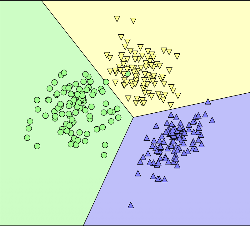
Explanation

The boundary between regions $R_k$ and $R_j$ is where $y_k(x)=y_j(x)$:

$$(w_k-w_j{)}^{\top }x+(w_{k_0}-w_{j_0})=0$$

This is itself a hyperplane, with normal vector $w_k-w_j$. There we have it. The boundary’s orientation depends on the difference of the two weight vectors, not on either one alone.

• The norm matters because each individual discriminant $y_k(x)=0$ doesn’t move if we rescale $w_k\to \alpha w_k,w_{k_0}\to \alpha w_{k_0}$, but the pairwise boundary $y_k(x)=y_j(x)$ becomes $(\alpha w_k-w_j{)}^{\top }x+(\alpha w_{k_0}-w_{j_0})=0$
  • As $\alpha$ changes, the normal $\alpha w_k-w_j$ rotates (unless perpendicular)

Tiny numeric example (2D, 2 classes)

We have $y_1(x)=x_1$, (i.e. $w_1=(1,0)$) and $y_2(x)=x_2$, (i.e. $w_2=(0,1)$)

Boundary is at $x_1=x_2\to$ the slope equals 1.

Now scale $w_1$ by $\alpha =2$, so $y_1(x)=2x_1$. The boundary now moves to $2x_1=x_2\to$ the slope equals 2.

Linear Perceptron

Inspired by the brain: binary signal, multiple inputs $\to$ one output, fires if activation is high enough.

The activation is defined by a non-linear step function:

$$f(x;w)=h(w^{\top }x)\text{, where }h(a)=\{\begin{array}{l}+1\text{, if a>0}\\ -1\text{ otherwise}\end{array}$$

The training dataset $\{x_n,t_n\}$ uses the target coding scheme:

$$t_n=\{\begin{array}{l}+1\text{, if }{x}_n\in C_1\\ -1\text{ otherwise}\end{array}$$

Training via stochastic gradient descent

Classification is correct if and only if:

$$w^{\top }{x}_n{t}_n>0$$

The objective is to minimize the misclassification rate $E(w)=-{\sum }_{n\in \mathcal{M}}{w}^{\top }{x}_n{t}_n$, where $\mathcal{M}=\{x_i\mid w^{\top }{x}_i{t}_i\le 0\}$ is the set of misclassified examples.

We simply update the weights by sgd:

$$\begin{array}{rl}{w}^{(i)}& =w^{(i-1)}-\eta {\nabla }_{w}E(w^{(i-1)})\\ & =w^{(i-1)}+\eta \sum _{n\in \mathcal{M}}{x}_n{t}_n\\ & \approx w^{(i-1)}+\eta \cdot x_n\cdot t_n\text{ for some n where }{w}^{\top }{x}_n{t}_n<0\end{array}$$

that’s the “stochastic” part — one misclassified example per update rather than the full batch. It reads as “whenever you hit one that’s misclassified, nudge $w$ in the direction of $x_n{t}_n$ scaled by $\eta$. Repeat until no misclassifications remain.”

Perceptron Convergence Theorem

If the training set is linearly separable, the algorithm is guaranteed to find a solution in a finite number of steps.

Problems with perceptrons

• slow, doesn’t generalize past 2 classes, no way to tell “not separable” from “slow to converge”, not guaranteed to reduce error every step (the set of misclassified training examples changes at each weight update), solution depends on initial conditions.

Gradient Descent flavors

• Batch: sum over all data points
• Stochastic: approximate with one random point at a time — fast, avoids bad local optima, handles redundancy; but noisy, messier stopping criterion
• Minibatch: sum over a subset

Probabilistic Models

they can deal with missing data, include prior knowledge and uncertainty in our parameter values. Confidence comes as a prediction.

Generative Probabilistic Models

Learn the point $p(x,C)$, classify via Bayes’ rule:

$$p({\mathcal{C}}_i|\mathbf{x})=\frac{p(\mathbf{x}|{\mathcal{C}}_i)p({\mathcal{C}}_i)}{{\sum }_{k}p(\mathbf{x}|{\mathcal{C}}_k)p({\mathcal{C}}_k)}$$

• it’s optimal as long as the true distributions are learned correctly as $n\to \infty$.
• for certain distributions, the model results in linear classification.
  • an example would be normal distributions with shared covariances: ${\sum }_k={\sum }_i$.

Demonstration

The decision boundary between two classes ${\mathcal{C}}_k$ and ${\mathcal{C}}_j$ occurs where their posterior probabilities are equal:

$$p({\mathcal{C}}_k|\mathbf{x})=p({\mathcal{C}}_j|\mathbf{x})⟺\ln \frac{p(\mathbf{x}|{\mathcal{C}}_k)p({\mathcal{C}}_k)}{p(\mathbf{x}|{\mathcal{C}}_j)p({\mathcal{C}}_j)}=0$$

For a multivariate Gaussian distribution with class mean ${\mathbf{\mu }}_k$, shared covariance matrix ${\mathbf{\Sigma }}_k=\mathbf{\Sigma }$, and input feature dimension $D$ (where $\mathbf{x}\in {\mathbb{R}}^D$):

$$p(\mathbf{x}|{\mathcal{C}}_k)=\frac{1}{(2\pi {)}^{D/2}|\mathbf{\Sigma }{|}^{1/2}}\exp \left(-\frac{1}{2}(\mathbf{x}-{\mathbf{\mu }}_k{)}^{\top }{\mathbf{\Sigma }}^{-1}(\mathbf{x}-{\mathbf{\mu }}_k)\right)$$

Taking the logarithm:

$$\ln p(\mathbf{x}|{\mathcal{C}}_k)=-\frac{1}{2}{\mathbf{x}}^{\top }{\mathbf{\Sigma }}^{-1}\mathbf{x}+{\mathbf{\mu }}_k^{\top }{\mathbf{\Sigma }}^{-1}\mathbf{x}-\frac{1}{2}{\mathbf{\mu }}_k^{\top }{\mathbf{\Sigma }}^{-1}{\mathbf{\mu }}_k-\frac{1}{2}\ln |\mathbf{\Sigma }|-\frac{D}{2}\ln (2\pi )$$

Because all classes share the exact same covariance $\mathbf{\Sigma }$, the quadratic term $-\frac{1}{2}{\mathbf{x}}^{\top }{\mathbf{\Sigma }}^{-1}\mathbf{x}$ and the normalization constants $-\frac{1}{2}\ln |\mathbf{\Sigma }|-\frac{D}{2}\ln (2\pi )$ are identical.

Subtracting the log-likelihoods cancels out the quadratic ${\mathbf{x}}^{\top }{\mathbf{\Sigma }}^{-1}\mathbf{x}$ component completely:

Setting the log-posterior ratio to zero yields a purely linear boundary ${\mathbf{w}}^{\top }\mathbf{x}+w_0=0$:

$$\mathbf{w}={\mathbf{\Sigma }}^{-1}({\mathbf{\mu }}_k-{\mathbf{\mu }}_j)$$

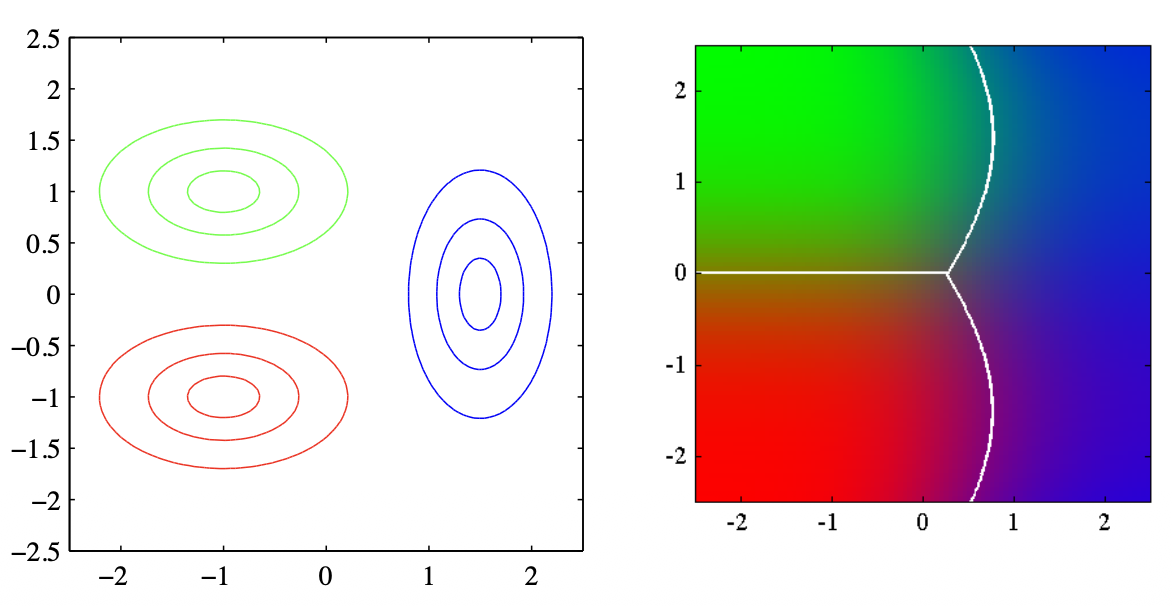
Discriminative Probabilistic Models

1. We directly optimize $p(C_k\mid x)$ instead of modelling $p(x,C)$. They model the posterior distribution $p(C_k\mid x)$ for a two-class problem as a sigmoid $\sigma (a)=\frac{1}{1+e^{-a}}$ (goes from 0 to 1, and at $a=0$, we go through 0.5).

$$\begin{array}{rl}p({\mathcal{C}}_1|\mathbf{x})& =\frac{p(\mathbf{x}|{\mathcal{C}}_1)p({\mathcal{C}}_1)}{p(\mathbf{x}|{\mathcal{C}}_1)p({\mathcal{C}}_1)+p(\mathbf{x}|{\mathcal{C}}_2)p({\mathcal{C}}_2)}\\ & =\frac{1}{1+\frac{p(\mathbf{x}|{\mathcal{C}}_2)p({\mathcal{C}}_2)}{p(\mathbf{x}|{\mathcal{C}}_1)p({\mathcal{C}}_1)}}\\ & =\sigma (a(\mathbf{x}))\text{where }a(\mathbf{x})=-\ln \frac{p(\mathbf{x}|{\mathcal{C}}_2)p({\mathcal{C}}_2)}{p(\mathbf{x}|{\mathcal{C}}_1)p({\mathcal{C}}_1)}\end{array}$$

2. For $K$ classes, the posterior is a softmax function: $p(C_k\mid x)=\frac{exp(a_k)}{{\sum }_{j}exp(a_j)}$:

To derive the $k$-class posterior, start with Bayes’ theorem to find the probability of class $C_k$ given data $\mathbf{x}$:

$p(C_k|\mathbf{x})=\frac{p(\mathbf{x}|C_k)p(C_k)}{p(\mathbf{x})}$

Expand the marginal probability in the denominator over all possible $j$ classes using the law of total probability:

$p(C_k|\mathbf{x})=\frac{p(\mathbf{x}|C_k)p(C_k)}{{\sum }_{j}p(\mathbf{x}|C_j)p(C_j)}$

Define the activation $a_k$ as the natural logarithm of the joint probability:

$a_k=\ln \{p(\mathbf{x}|C_k)p(C_k)\}$

Take the exponential of both sides to express the joint probability in terms of $a_k$:

$\exp (a_k)=p(\mathbf{x}|C_k)p(C_k)$

Substitute this exponential form into both the numerator and the sum in the denominator to yield the final softmax function for $k$ classes:

$p(C_k|\mathbf{x})=\frac{\exp (a_k)}{{\sum }_j\exp (a_j)}$

for 2 classes $\to$ sigmoid, for K-classes $\to$ softmax.

Generative vs. Discriminative

Generative models learn the distribution of the data:

• can sample/generate data
• optimal if known true distribution

Discriminative models directly optimize $p(C_k\mid x)=\sigma (a(x))$:

• a is linear in case of normal distributions with shared covariances
• more robust when true distributions are unknown
• requires more data.

Logistic Regression

We wrote the posterior probability of the class given a datapoint as:

$$\begin{array}{rl}p(c_1\mid \mathbf{x})& =\sigma (\mathbf{w}\cdot \mathbf{x})\\ p(c_2\mid \mathbf{x})& =1-p(c_1\mid \mathbf{x})\end{array}$$

The parameters of this model, $\mathbf{w}$, can be trained by conditional Maximum Likelihood:

$$\begin{array}{rl}{\mathbf{w}}^{\ast }& =\arg \underset{\mathbf{w}}{\max }\prod _{i}p(c_i\mid {\mathbf{x}}_i)\\ & =\arg \underset{\mathbf{w}}{\max }\prod _i\sigma (\mathbf{w}\cdot {\mathbf{x}}_i{)}^{y_i}{\left(1-\sigma (\mathbf{w}\cdot {\mathbf{x}}_i)\right)}^{1-y_i}\end{array}$$

This is equivalent with minimizing the binary cross-entropy loss. Taken from Contextual Word Embeddings and Transformers.

Basic Functions

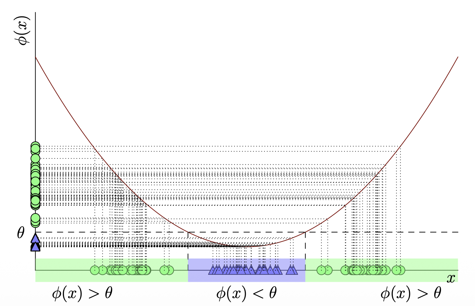
Linear models might be restricted, but they are cheaper to train and less prone to overfitting due to their few adjustable parameters.

We keep the advantage of the classifiers and extend to non-linear problems by transforming the features:

$$x\to \varphi (x),w^{\top }x\to w^{\top }\varphi (x)$$

“Linear” here means linear in parameters, not in data.

The model is still calculating a simple weighted sum using the parameters w, which makes it mathematically a linear model that is easy to train and less prone to overfitting. However, instead of applying these weights to the raw data $x$, it applies them to the transformed features $\varphi (x)$. This means the model is no longer linear with respect to the original input space, allowing it to capture complex, non-linear patterns while keeping the underlying parameter optimization simple.

Gaussian basis functions reshape the feature space to make the classes separable

No single straight line can successfully split the two groups in the left image. By feeding this raw data through non-linear Gaussian basis functions centered at specific points like ${\mu }_1$​ and ${\mu }_2$​, the data is projected into an entirely new coordinate system defined by ${\varphi }_1$​ and ${\varphi }_2$​.

This mathematical transformation warps the space so that the red dots cluster together at the top and the blue dots group at the bottom (right image). Once the data is reshaped into this new space, a standard linear classifier can easily draw a straight line to separate the classes.

Regularization (dealing with overfitting)

The problems are:

1. more basis functions $\to$ more parameters $\to$ risk of overfitting
2. lacking the right basis functions $\to$ insufficiently flexible model (underfitting)

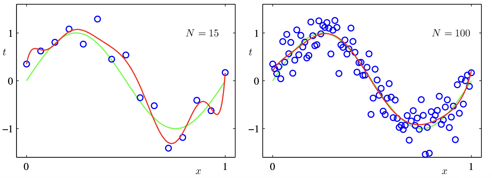
If we revisit the polynomial regression $y=w_0+w_{1}x+w_2{x}^2+\dots$ (rewrite $x$ as basis function) example where we try to fit the sin function $y=sin(2\pi x)$ where the observations are corrupted by Gaussian noise and we minimize the error function:

$$\hat{E}(w)=\frac{1}{2}\sum _{n=1}^N(y(x_n,w)-t_n{)}^2$$

We observe that increasing the model complexity $M\to \infty$, we overfit the noise.

Complete from slide 37/41.