Mobile Laser Scanning (MLS)

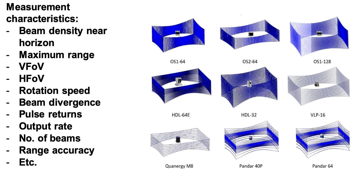
The vertical resolution of a LiDAR sensor depends on the number of laser channels and their angular separation. Multiline LiDARs use multiple laser channels fixed at different vertical angles to acquire 3D data per rotation. The effective range of a LiDAR sensor depends on the reflectivity of targets and the power of the laser pulse. Accuracy typically decreases with increasing range due to beam divergence, angular error, and timing jitter. The primary strength of MLS compared to the other strategies is Geometry. Ghost points in MLS are mainly caused by reflections from glass.

MLS combines

• Laser scanner for 3D data acquisition
• GNSS/IMU for positioning and orientation
• Platform (car, boat, UAV, backpack)
• Cameras for visual context (optional)

Add the application for each to the bullet points, you have in slides

The key advantage is the continuous data collection while moving $\to$ dense, accurate 3D data at ground level. The key challenge is the sensor fusion and the drift that accumulates.

The range is smaller, since we are close to the scenes, so we also have better point density distribution.

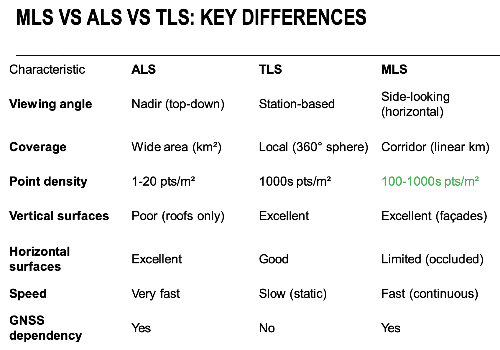
MLS vs. ALS vs. TLS

TLS > MLS > ALS in terms of point density.

Again, based on TOF (time of flight)

$$range=\frac{c(t_2-t_1)}{2}$$

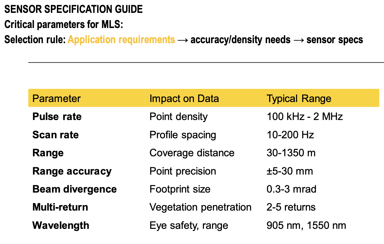
Multi-return capability: One pulse can generate 2-5 returns $\to$ Essential for vegetation penetration (it’s the idea that the waves could scatter when they hit some surfaces and then they reflect back. you know it, the idea with the airport as well with gnss and clouds).

Multi-beam lidars are mostly used in autonomous driving because they are cheaper. Single-beam is mostly used when you need high-quality point cloud.

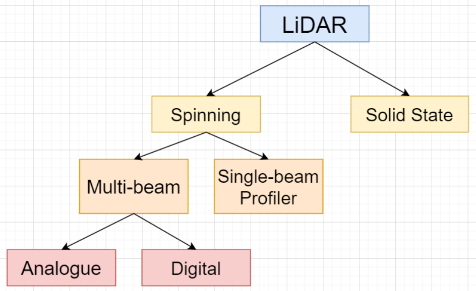
Multi-beam spinning LiDARs

• VLP-16 is for example cheaper and it offers bad point density distribution. (attach the image)
• Pandar 40P is mostly used in autonomous driving because it assigns some importance to the direct horizontal view, but also up and down.

Sensor Specification Guide

For myself, some explanations:

• Pulse rate is the number of individual laser pulses emitted by the sensor per second.
• Scan rate (or frame rate) refers to how quickly the sensor’s scanning mechanism moves the laser beam across its field of view

So the pulse rate tells you how many points are being fired, the scan rate tells you how quickly the sensor is covering its entire viewing area.

• Wavelength determines how much interference the sensor faces from the sun. Many LiDARs operate at 905 nm because components are inexpensive, but this spectrum contains significant solar “noise.” Moving to 1550 nm allows the sensor to operate in a region where the atmosphere absorbs more solar radiation, providing a cleaner signal-to-noise ratio. Additionally, certain wavelengths penetrate fog, rain, or dust more effectively than others.
  • Different surfaces reflect light differently based on the wavelength. For example, vegetation reflects Near-Infrared (NIR) light very strongly, which is why 905 nm or 1064 nm lasers are excellent for mapping forestry or biomass.

Point Density Calculation Framework

So we know the LiDAR has the Emitter and a rotating mirror. What happens then is the beam successfully reflects the beams in a 2D circular manner.

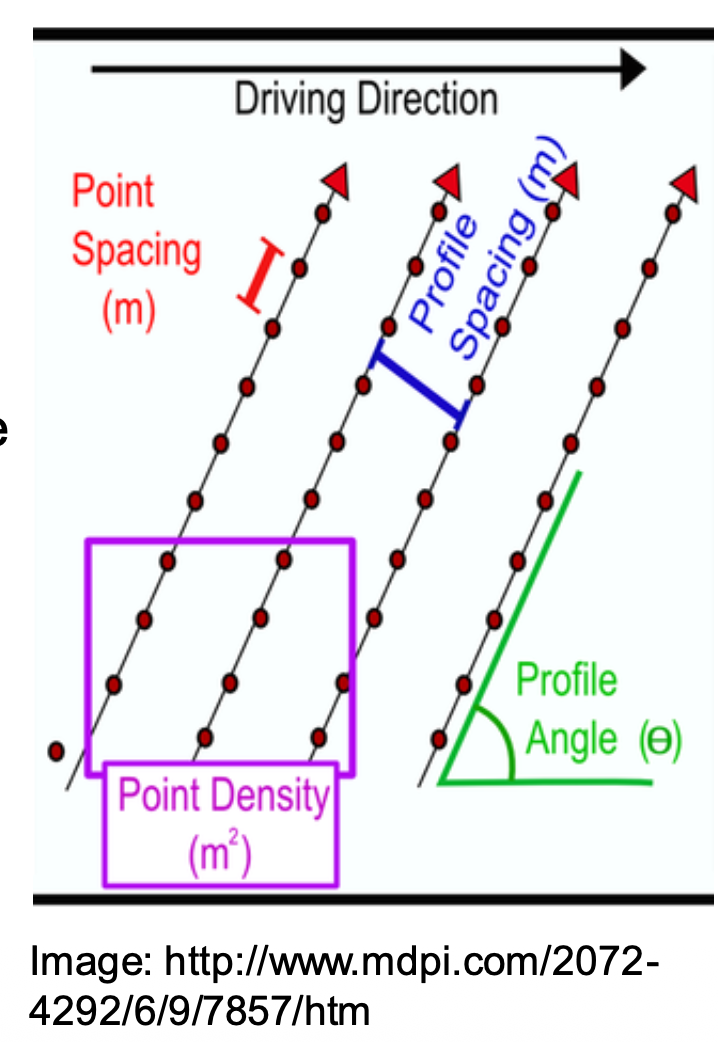
Along-track Profile Spacing ($d_{\text{along}}[m]$)

This is the gap between the parallel lines (scan lines) that the LiDAR draws as the vehicle moves forward. We talk about driving direction and scan profile(the green one). Each time the mirror rotates a little bit, we get to the next point position (the red dots).

$$d_{\text{along}}=v/f_{scan}[\text{i.e. profile spacing}]$$

• $v$ is the platform speed
• $f_{\text{scan}}$ is the scan frequency (i.e. scan rate)
• If the scanner spins at a fixed frequency, but the vehicle drives faster, the lines will be stretched further apart.

Cross-track Point Spacing ($d_{\text{across}}[m]$​)

This is the gap between individual laser dots within a single scan line (distance between the red dots). The formula is calculating the arc length of the scan.

$$d_{\text{across}}=\frac{2\pi r{f}_{scan}}{f_{pulse}}[\text{i.e. point spacing}]$$

• $f_{pulse}$ is the pulse rate
• $r$ is range to target

Point Density ($\rho [pts/m^2]$)

• It is simply the inverse of the area of the rectangle formed by your along-track and cross-track spacing.

$$\rho =\frac{1}{d_{\text{across}}\cdot d_{\text{along}}}$$

Example

• The platform drives at $v=50[km/hr]$
• The lidar does 100 full rotations each second ⇒ $f_{\text{scan}}=100[Hz]$
• In 1 second we expect to get 1 million returns ⇒ $f_{\text{pulse}}=1[MHz]$
• We consider the range to target as $r=100m$.

Therefore, $d_{\text{along}}=\frac{13.89(m/s)}{100(Hz)}=0.14[m]$.

And then $d_{\text{across}}=\frac{2\pi \cdot 100(m)\cdot 100(Hz)}{1,000,000(Hz)}=0.06[m]$

In the end, $\rho =\frac{1}{0.14(m)\cdot 0.06(m)}=120[pts/m^2]$

Some characteristics of MLS is that it varies in point density. It depends on multiple key factors:

1. Range Dependency
   1. Ofc, you can keep the speed constant, but in real-life it’s not highly realistic.
   2. Far objects get exponentially lower density
2. Speed Dependency
   1. $2\times$ speed $\to$ $2\times$ along-track spacing $\to \frac{1}{2}$ density
3. Occlusions
4. Scan angle
   1. Perpendicular surfaces: maximum density

So if at $v=50[km/hr]$ I get $\rho =120[pts/m^2]$

• At $20[km/hr]$, the density becomes $\rho =300[pts/m^2]$.
• At $100[m]$ range vs $10[m]$: $10\times$ difference in cross-track spacing!

You can calculate what factors you need to have a set point density $\rho$.

How many points per $m^2$ are needed to detect a 5cm height difference from the road to the pedestrian walk?

Intuitively, it would come down to $d_{\text{across}}$ to be smaller than the height of the object.

Advantages:

• Excellent vertical surface coverage (building façades)
• 360 degrees data (with multiple scans)

Disadvantages:

• Roof surfaces are rarely visible (use ALS for fusion)
• No dense vegetation representation due to laswer power limitations

YOU CAN COMBINE MLS AND ALS into one combined point cloud. MLS could see the traffic lines very well, and the ALS could complete the roof of buildings, crowns of trees, etc. To match them, you need to go to the 3D bird-eye-view projection of the MLS and then match the features with the pov of the ALS (done in practice).

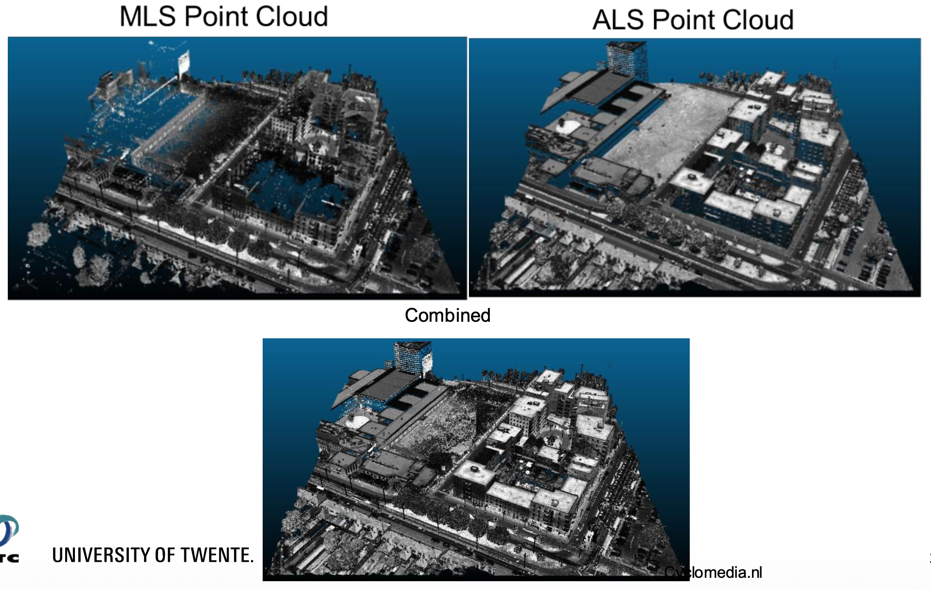
look over the questions: https://app.wooclap.com/XFXFMA/questionnaires/69899832cb269fc22c653f64. You have the pictures saved on your desktop.

In the density visualization (rainbow colored image), why are the floor areas showing higher point density (yellow/green) compared to the walls (blue)?

From Claude: In MLS, the scanner is mounted on a vehicle moving along the road. The laser beams hit the floor at a near-perpendicular incidence angle across the entire trajectory, accumulating many points with each pass. Walls are only hit at grazing angles from the side, receiving far fewer points.

What is survey grade? What’s the difference to mapping grade? Is it the precision?

• Survey grade (GNSS/positioning): typically <2 cm accuracy, often post-processed or RTK-corrected, used for legal/cadastral work.
• Mapping grade: typically 0.5–2 m accuracy, sufficient for GIS mapping and inventory but not for precise boundary or engineering work.

We can down-sample the point cloud? Does that mean I always want as much as possible and discard what I don’t need?

Remember from Global Navigation Satellite System (GNSS) that if you are between two tall buildings, the GNSS signal bounces a lot between them until it reaches my terminal. This is one of the disadvantages in MLS.

UAV-based MLS are handy in powerline inspection. I guess it’s not ALS since the point density is not as bad ($\rho \sim 50-200points/m^2$)

How does LiDAR deal with transparent windows?

• They create outliers. Pretty much an edge case for LiDARs. Look over it more because his explanation made pretty much no sense.

How does LiDAR see text on a plate?

• is it intensity based?

A nice emerging trend is the digital twins — you scan and make a digital representation of something from reality. Especially applied in virtual cities I guess.

Look over the exercise provided by Ville

• Reading material: Puente, I., González-Jorge, H., Martínez-Sánchez, J., & Arias, P. (2013). Review of mobile mapping and surveying technologies. Measurement, 46(7), 2127-2145. link

Possible EXAM questions

---

• Compare ALS, TLS, and MLS in terms of (i) acquisition geometry, (ii) point density characteristics, (iii) positioning accuracy, and (iv) typical applications. For each method, list one key advantage and one key limitation.

	ALS	TLS	MLS
Acquisition geometry	Airborne, nadir/oblique, large swath	Static, tripod-mounted, 360° from fixed positions	Mobile platform (car/rail), side-looking along corridor
Point density	Low–medium (1–50 pt/m²)	Very high (thousands pt/m²)	High (100–1000 pt/m²)
Positioning accuracy	10–30 cm (GNSS/IMU from altitude)	2–6 mm (no GNSS needed, stable platform)	3–10 cm (GNSS/IMU dependent)
Typical applications	Terrain/DTM, forestry, flood modelling	Heritage, structural inspection, indoor	Road mapping, urban corridors, infrastructure
Key advantage	Massive area coverage quickly	Highest geometric accuracy and density	Fast corridor mapping at street level
Key limitation	Poor detail on vertical surfaces, weather dependent	Slow, labor-intensive, no large-area coverage	GNSS-dependent, degrades in urban canyons

---

• Given an MLS application of your choice (e.g. road inventory or urban mapping), outline a survey plan addressing: (i) sensor configuration, (ii) trajectory design, (iii) reference data requirements, and (iv) expected challenges.

Road Inventory - MLS Plan

(i) Sensor Configuration

• LiDAR: $2\times$ multiline LiDAR (e.g. Velodyne VLP-32C), mounted left/right at ~45° tilt to capture road surface, curbs, signs, and façades
• GNSS: dual-frequency receiver for RTK positioning
• IMU: tactical-grade, tightly coupled with GNSS
• Cameras: optional, for sign recognition and texture

(ii) Trajectory Design

• Drive each lane twice in opposite directions to reduce occlusion
• Speed: 30–50 km/h (faster = lower density)
• Overlap between adjacent strips for redundancy
• Avoid peak traffic hours to reduce dynamic object interference

(iii) Reference Data Requirements

• GCP (Ground Control Points): retroreflective targets placed every ~500m for georeferencing validation
• GNSS base station within 10–15 km for differential correction
• IMU calibration: pre-survey figure-8 maneuver to initialize IMU orientation

(iv) Expected Challenges

• Urban canyons: GNSS multipath $\to$ mitigated by IMU bridging and SLAM-based post-processing
• Dynamic objects: cars, pedestrians create noise $\to$ filtered by intensity/temporal consistency
• Occlusion: parked vehicles block curbs/signs $\to$ solved by multi-pass and opposite-direction drives
• Data volume: high pt density = large storage and processing requirements

---

• Explain why MLS point clouds exhibit non-homogeneous point density. Your answer should reference sensor geometry, platform motion, and scene structure.

Point density in MLS is the result of three interacting factors:

Sensor geometry The scanner rotates and emits pulses at fixed angular intervals, meaning point spacing increases with distance from the scanner. Objects close to the vehicle get hit by many beams at near-perpendicular angles; objects far away or at grazing angles receive far fewer points. Vertical surfaces like walls are inherently undersampled compared to horizontal surfaces like roads.

Platform motion As the vehicle moves, the scanner’s position shifts between each rotation. At low speed, consecutive scan profiles overlap heavily $\to$ high density. At high speed, profiles are spread further apart $\to$ lower density. Curves and intersections where the vehicle slows down naturally produce denser regions. Along straight highways at constant speed, density is more uniform but lower overall.

Scene structure Occluding objects (parked cars, trees, street furniture) block laser pulses from reaching surfaces behind them, creating shadow zones with zero or near-zero density. Building corners, overhangs, and narrow alleys compound this. Highly reflective surfaces (glass, metal) can cause pulse saturation or spurious returns, locally distorting apparent density.

Combined effect The result is that density varies systematically with distance from trajectory, vehicle speed, and scene complexity — meaning a single MLS pass almost never produces uniform coverage, which is why multi-pass and opposite-direction drives are standard practice.

---

• Given a platform and a setting, calculate the required MLS point cloud surface density. I’ve done that already in the example.

---

• What are the advantages and challenges of MLS considering the following applications: Roads, Urban, Indoor, Forest.

• Roads: MLS is the ideal tool — environment matches the acquisition geometry perfectly
• Urban: MLS works well but GNSS reliability is the bottleneck
• Indoor: GNSS-denied → requires LiDAR SLAM or wheel odometry; positional drift is the main enemy
• Forest: MLS is the weakest fit — canopy occlusion and rough terrain make it difficult; ALS or UAV-LiDAR often preferred instead