Data Exploration & Preprocessing

• Data Exploration — visualizing only, non-invasive (always safe to redo)
  • tells me what needs fixing
• Data pre-processing — cleaning, imputing, invasive i.e. changing the data itself
  • does the fixing

Garbage in, Garbage out

One bad row can distort a mean, a plot, or a trained model. A model or chart is only as trustworthy as the data behind it.

The six dimensions of data quality

1. Completeness — are values missing? (e.g. a blank lab value)
2. Accuracy — are values correct? (e.g. recording a patient’s blood type as A+ when they are actually O-)
3. Consistency — do values agree across the dataset? (e.g. “NL” and “Netherlands” in the same column)
4. Validity — do values respect allowed ranges or formats? (e.g. a negative age or a birth year of 1899)
5. Uniqueness — are there duplicate records? (e.g. same patient recorded twice)
6. Timeliness — is the data current enough to use? (e.g. relying on a patient’s contact information from five years ago to send an urgent appointment reminder today, meaning the data is no longer current enough to be useful)

Series are 1-D (age column) and DataFrames are 2-D (age,city). I.e. a DataFrame is a table, each column is a Series.

df = pd.DataFrame({
	"name": ["Ana", "Bo", "Cy"],
	"age": [23, 45, 31],
})
 
print(df.shape) _# (3, 2)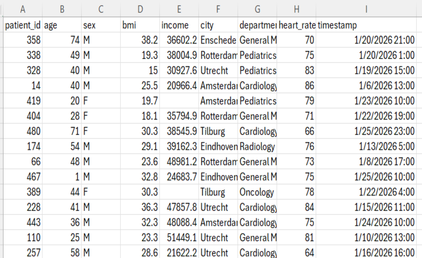

yes, I trust I am enough of an idiot to mix them.

Data types matter

• Numeric — continuous (age, income) or discrete (counts)
• Categorical — a fixed set of labels (blood type, country)
• Datetime — timestamps, dates, durations

Descriptive Statistics

Mean — the arithmetic average; sensitive to outliers

Median — the middle value; robust to outliers

• It is calculated by arranging all the numbers in numerical order and selecting the exact middle number, or averaging the two middle numbers if there is an even amount of values.

Mode — the most frequent value; useful for categorical data

Compare mean and median to spot skew at a glance

Skew refers to the asymmetry of a data distribution.

Rule of thumb: If the mean is greater than the median, the data has a right skew because high outliers pull the average up. If the mean is less than the median, the data has a left skew because low outliers pull the average down.

For a right skew, consider the odd-length series 1, 2, 2, 3, and 20. The median is the exact middle number, which is 2. The mean is the sum of all values divided by 5, which is 5.6. Since the mean of 5.6 is greater than the median of 2, the high outlier pulls the average up, creating a right skew.

For a left skew, consider the even-length series 1, 15, 16, 17, 18, and 19. Because the series has an even number of values, the median is the average of the two middle numbers (16 and 17), which is 16.5. The mean is the sum of all values divided by 6, which is approximately 14.33. Since the mean of 14.33 is less than the median of 16.5, the low outlier pulls the average down, creating a left skew.

Measures of spread

Variance — average squared distance from the mean

$${\sigma }^2=\frac{\sum (x_i-\mu {)}^2}{N}$$

Standard deviation — variance in the original units

$$\sigma =\sqrt{{\sigma }^2}$$

Z-standardization refers to rescaling data so that it has a mean of 0 and a standard deviation of 1, which is calculated using the equation:

$$z=\frac{x-\mu }{\sigma }$$

Normalization: often referred to as Min-Max scaling, differs from standardization by rescaling the data to fit within a specific, fixed range, typically between 0 and 1. While standardization centers the data around a mean of 0 with a standard deviation of 1 without bounding the extreme values, normalization shifts and compresses all values into the [0, 1] interval, making it highly sensitive to outliers. The equation for normalization is:

$$x_{norm}=\frac{x-x_{min}}{x_{max}-x_{min}}$$

Quartiles & IQR — the middle 50% of the data

$$IQR=Q3-Q1$$

Range — max minus min; very sensitive to outliers

$$Range=x_{max}-x_{min}$$

Spread tells you how much to trust the central value.

.describe()

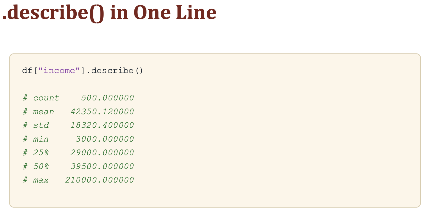
• the output provides summary statistics for 500 income records. I can determine that the data has a right skew because the mean of 42350.12 is greater than the median (50%) of 39500.00. This skew is likely driven by high outliers, given that the maximum income is 210000, which is vastly larger than the median. Additionally, the standard deviation of 18320.40 indicates a significantly wide spread in the recorded incomes.

---

Box plots: Spread & Outliers

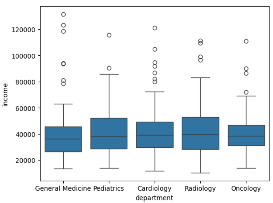
Five numbers: min, max, median, Q1, Q3

• the box marks Q1-Q3, so the middle 50% of the data
• the line inside the box is the median
• points beyond the whiskers are flagged as outliers

The whisker actually represents the maximum non-outlier value, rather than the absolute maximum of the entire dataset.

Here is how those whisker limits are standardly calculated (often called Tukey’s fences):

• First, find the Interquartile Range (IQR), which is the distance between the ends of the box (Q3 - Q1).

• The theoretical upper boundary is Q3 + (1.5 * IQR).

• The theoretical lower boundary is Q1 - (1.5 * IQR).

The whisker is drawn out to the highest actual data point in your dataset that still falls inside that upper boundary. Any data points that are higher than that 1.5 * IQR limit are classified as outliers and plotted as individual dots. So, in the context of a box plot, “min” and “max” really mean the lowest and highest typical values before reaching outlier territory.

Violin plots

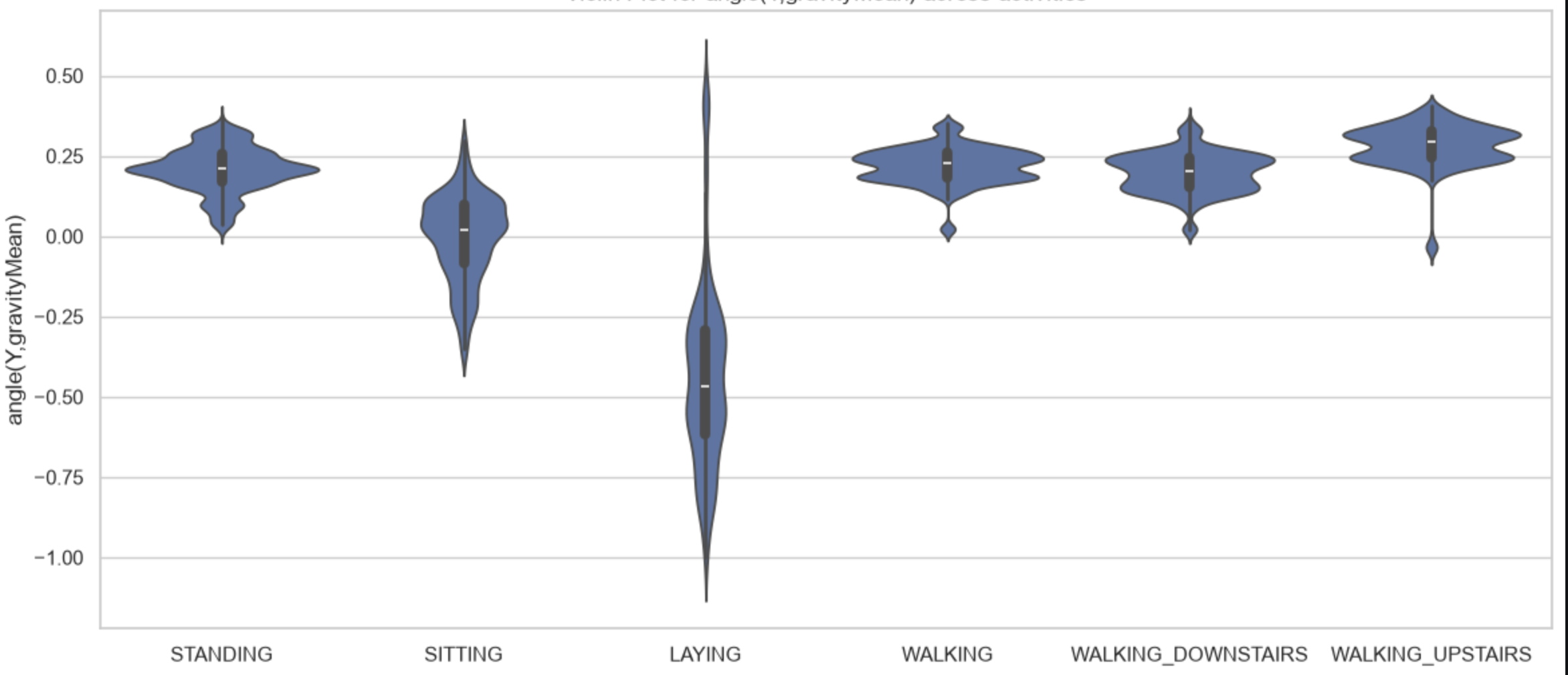
In a violin plot, a wider section means higher data density i.e. more common values and narrower sections represent lower data density i.e. rarer values.

Correlation matrix

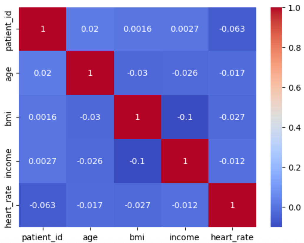
values close to +1 or -1 indicate a strong linear relationship. However, looking at the provided matrix, the intersections between patient_id, age, bmi, income, and heart_rate are all colored deep blue with values very close to 0 (ranging from -0.1 to 0.02). This indicates that there are no strong linear relationships between any of these specific features in this dataset.

---

Cleaning your data

Finding duplicates

A single row recorded twice skews every statistic.

df.duplicated().sum() # how many?
 
df[df.duplicated()] # which rows?
 
df = df.drop_duplicates() # Always inspect duplicates before dropping them — sometimes they're legitimate repeat visits

df = pd.read_csv("toy_data.csv")
unique_df = df[~df.duplicated()]
print(df.shape, unique_df.shape)
 
# Basically, the two duplicate rows got dropped.

Filtering with Constraints

# age can't be negative or over 120_
 
valid = df[(df["age"] >= 0) & (df["age"] <= 120)]
removed = len(df) - len(valid)
print(f"Dropped {removed} rows")

Detecting outliers — the IQR rule

Q1 = df["income"].quantile(0.25)
Q3 = df["income"].quantile(0.75)
IQR = Q3 - Q1
 
low, high = Q1 - 1.5*IQR, Q3 + 1.5*IQR
outliers = df[(df["income"] < low) | (df["income"] > high)]

Handling missing data

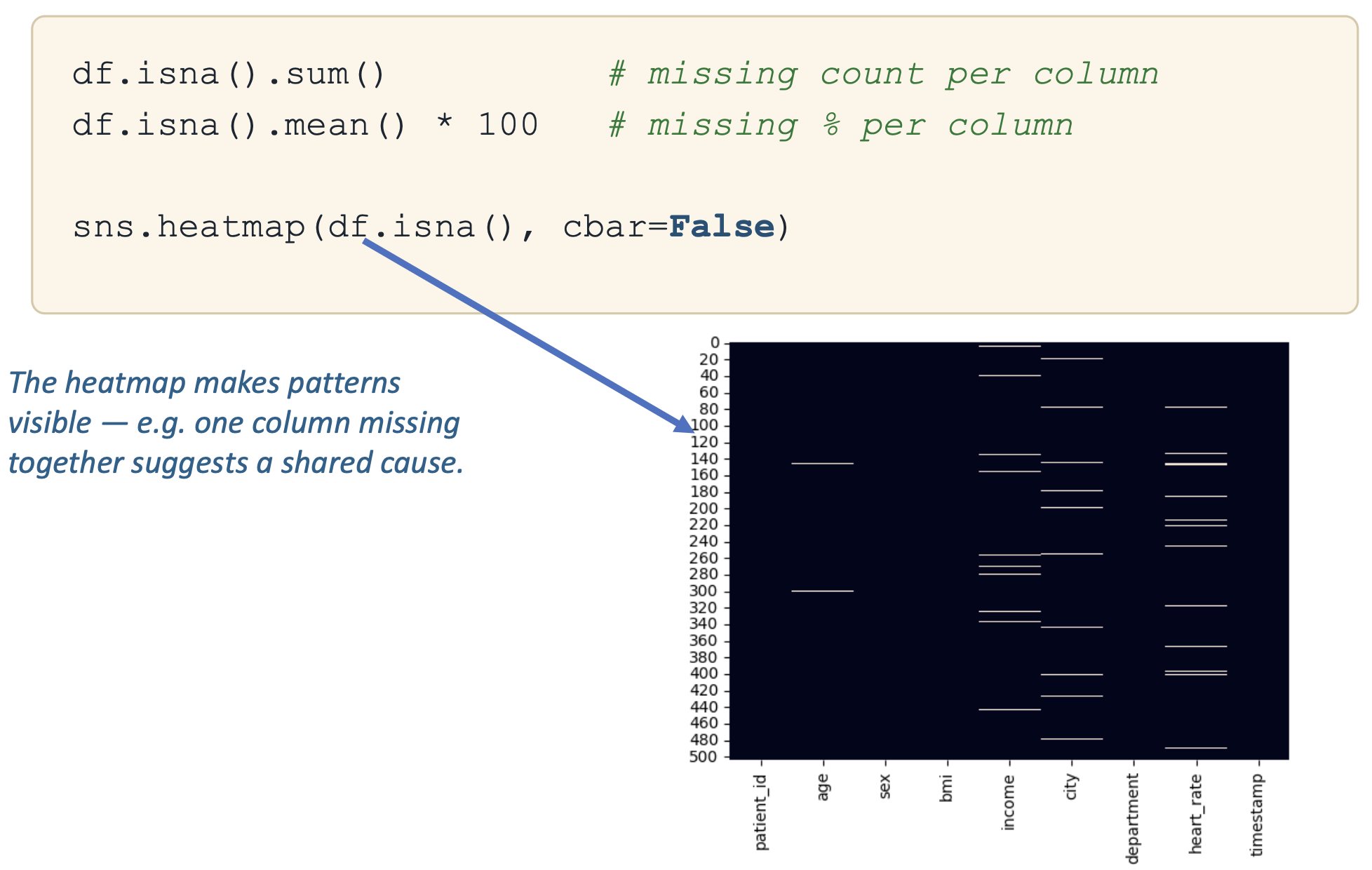
Imputation:

• fill with a representative value

# numeric column → median is robust to outliers
 
df["income"] = df["income"].fillna(df["income"].median())
 
# categorical column → most frequent value
 
df["city"] = df["city"].fillna(df["city"].mode()[0])

• carry the last known value forward-time dependent data

df = df.sort_values("timestamp")
df["heart_rate"] = df["heart_rate"].ffill()
 
# useful for sensor / time-series
# gaps — not for cross-sectional data

Cross-sectional data is information collected from multiple independent subjects or entities at a single, specific point in time, rather than tracking changes over a period. Because these records represent independent snapshots rather than a chronological sequence, time-dependent imputation methods like forward-filling are not suitable for this type of data.

imagine doing some experiment on a very hot day and the mobile phones heat or enter low-power mode and therefore the 50Hz is not guaranteed anymore. Any of these two could lead to incomplete datasets that would show up as NaN values.

• A technique I would use is imputation — filling missing values using a method like linear interpolation (reasonable for continuous sensor signals) or forward/backward fill for short gaps.

---

Scaling

• Columns on very different scales can dominate an analysis
  • Age (0–100) vs. income (0–200,000) — income would drown out age
• Many algorithms (distance-based, gradient-based) need comparable scales
  • Scaling changes the range, not the underlying relationships
• Rule of thumb: scale numeric features before feeding them to most ML models

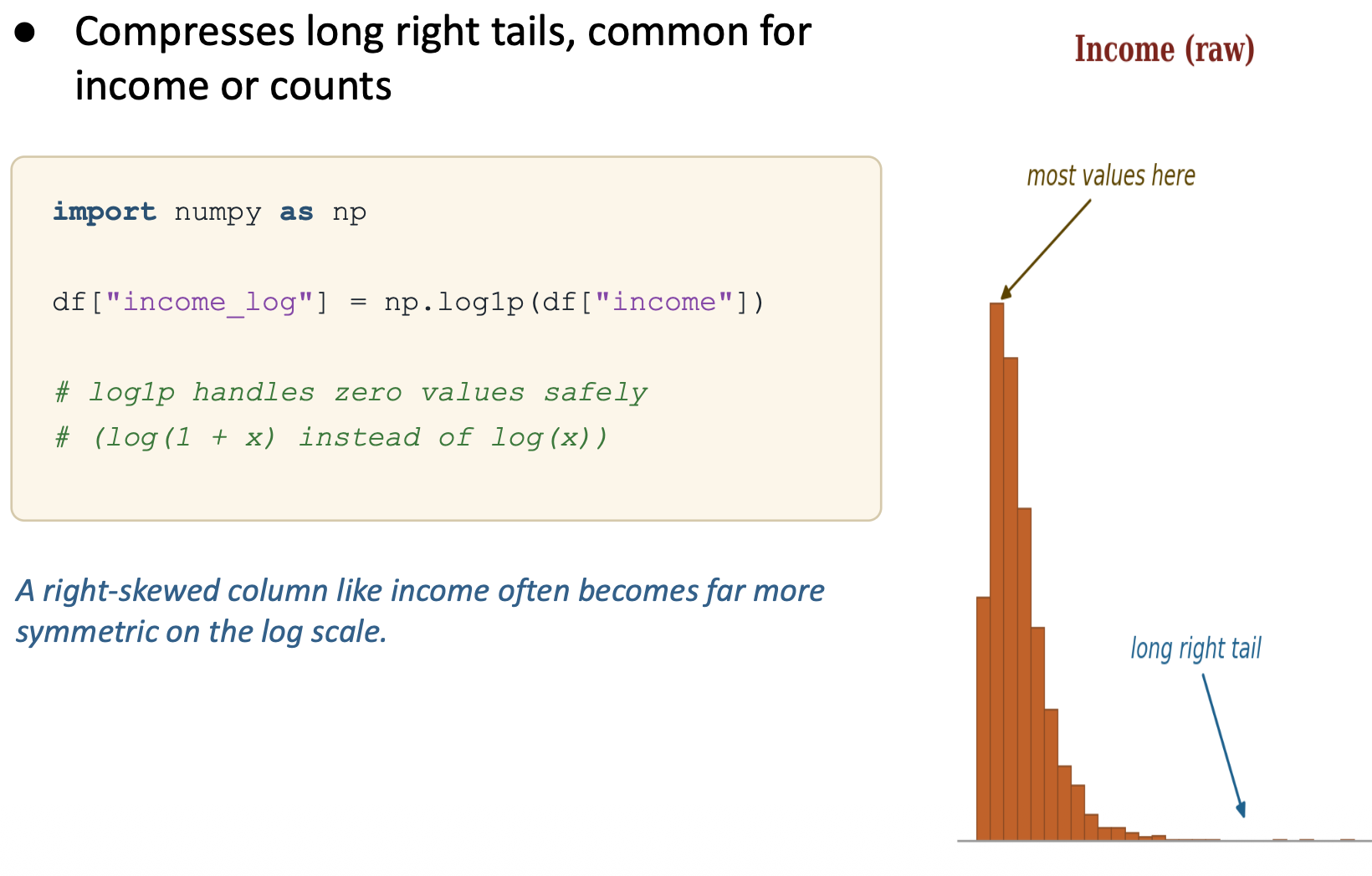
Log transform for skewed data as it compresses long right tails, common for income or counts

Careful: Avoiding Data Leakage. Fit scalers and imputers on the training set only Then apply (transform) the same fitted values to the test set. Fitting on the full dataset lets test information leak into training.

Rule of thumb: fit on train, transform on train and test

Encoding categorical values

• Most models need numbers, not text labels

# one-hot: a new 0/1 column per category
df = pd.get_dummies(df, columns=["city"])
 
# ordinal: use only when categories have order
sizes = {"small": 0, "medium": 1, "large": 2}
df["size_code"] = df["size"].map(sizes)

One-hot for unordered categories; ordinal only when the order itself is meaningful.

After applying one-hot encoding, the single Series no longer exists as a single column; it is transformed into a DataFrame (a table) containing multiple new columns, one for each unique category.

Index	City
0	Amsterdam
1	Utrecht
2	Eindhoven

After applying one-hot encoding, it looks like this:

Index	city_Amsterdam	city_Eindhoven	city_Utrecht
0	1	0	0
1	0	0	1
2	0	1	0

Merging tables — options

patients = pd.read_csv("patients.csv")
labs = pd.read_csv("lab_results.csv")
 
merged = pd.merge(patients, labs, 
					on="patient_id",
					how="left")

“on” names the shared key column; “how” decides which rows survive the merge.

• inner — keep only rows with a match in both tables
• left / right — keep all rows from one side, match where possible
• outer — keep every row from both sides
• Missing matches become NaN — often your next cleaning task
• Picking the wrong join type is a common, silent source of data loss

What would go wrong if one file wrote "WALKING" and another wrote "Walking", and you merged on that text column instead of the numeric code?

They would get treated as two different activities. I believe the rows would fail to match or even produce NaNs. I believe this is why matching based on a numeric scale (1-6) is safer than doing it on a string-based identifier, since they can include subtle inconsistencies.