Data Mining - Decision Tree Approach

The idea behind a decision tree is to repeatedly split the data into increasingly homogenous groups until a prediction can be made. To train a decision tree, we need a dataset containing an outcome variable and one or more predictors.

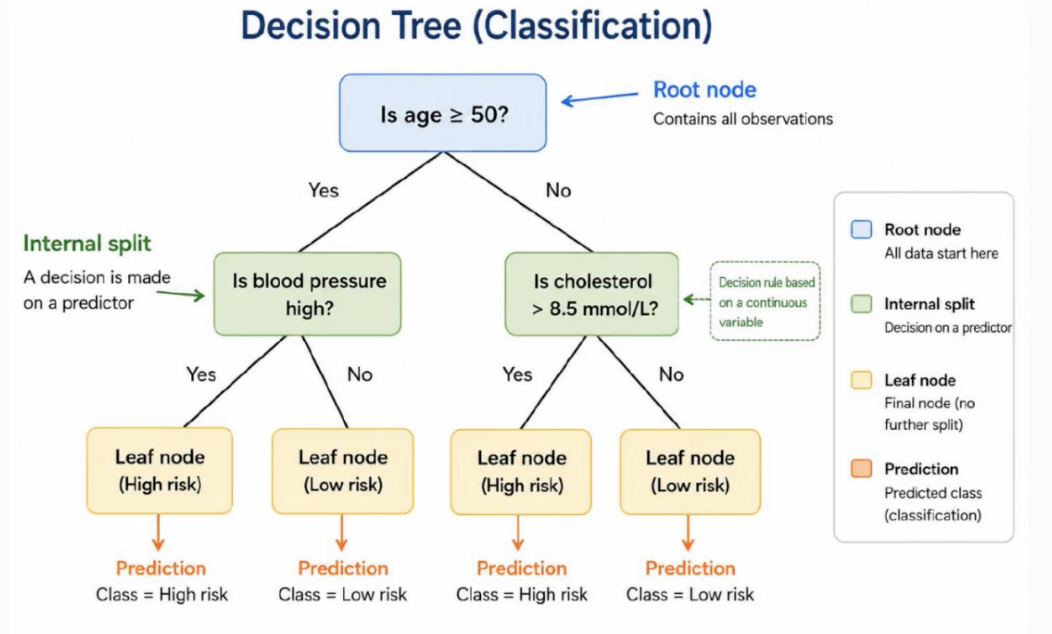
• when the outcome is categorical, we construct a classification tree.
• when the outcome is continuous, we construct a regression tree.
• the predictors are used to split the tree. It is okay to mix data types in the same tree.

We consider the person buying a computer example from the naive bayes approach. In that example we use 4 predictors: age, income, student status, and credit rating.

If we were to classify based on the age criteria, we would have 4 errors out of 14 observations:

• $\le 30$ would be classified as ‘NO’, but there are 2 in ‘YES’
• $31-40$ would be correctly classified as ‘YES’ with 0 errors
• $\ge 40$ would be classified as ‘YES’, but there are 2 in ‘NO’.

Based on this classification alone, the first split would be either age or student status.

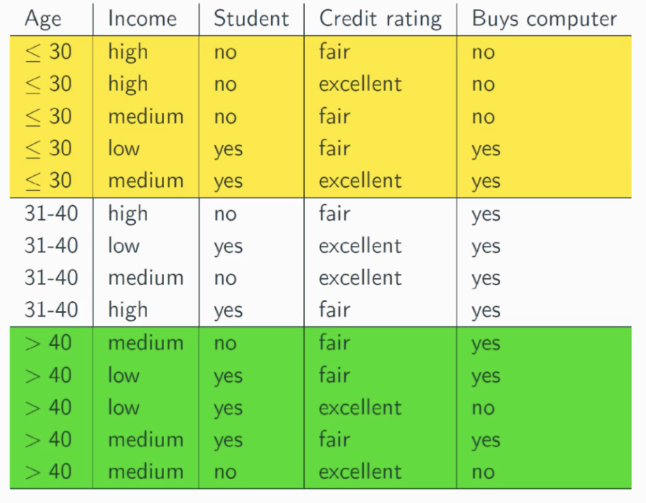
For example, if we include the student status for age, all people under 30 would be classified correctly. For 31-40 all are already classified as buyers.

In practice, however, we use other classification methods rather than simply selecting based on which class it falls in.

Gini index (for Classification)

• used to measure node purity in decision trees
• a node is pure if it contains only one class

$$gini(t)=1-\sum _j[P(j\mid t){]}^2$$

• where $P(j\mid t)$ is the relative frequency of class $j$ at node $t$.
• $gini(t)=0$ means it’s perfectly pure (all samples in one class)

• $gini(t)$ means more mixed classes.

Node contains 10 samples: 7 positive, 3 negative.

• $P(positive\mid t)=0.7$, $P(negative\mid t)=0.3$
• $gini(t)=1-(0.7^2+0.3^2)=0.42$
• interpretation: Node is impure because it contains mix of classes.

For a binary split like this one, 5/5 would be the worst case scenario since the classes would be equally mixed ⇒ $gini(t)=0.5$.

Example of Calculation Gini Index

Age	Yes	No	Total
≤30	2	3	5
31-40	4	0	4
>40	3	2	5
Total	9	5	14

$$gin{i}_{root}=1-(\frac{9}{14}{)}^2-(\frac{5}{14}{)}^2=0.46$$ $$gin{i}_{\le 30}=1-(\frac{2}{5}{)}^2-(\frac{3}{5}{)}^2=0.48$$ $$gin{i}_{31-40}=1-(\frac{4}{4}{)}^2-(\frac{0}{4}{)}^2=0$$ $$gin{i}_{>40}=1-(\frac{3}{5}{)}^2-(\frac{2}{5}{)}^2=0.48$$

$gin{i}_{age}=\frac{5}{14}\cdot 0.48+\frac{4}{14}\cdot 0+\frac{5}{14}\cdot 0.48=0.343$

And we can perform the same for the other predictors:

$$gin{i}_{student}=0.367$$ $$gin{i}_{income}=0.440$$ $$gin{i}_{rating}=0.429$$

age has the highest gini reduction (information gain): $0.46-0.343=0.116$, so age is chosen for the first split.

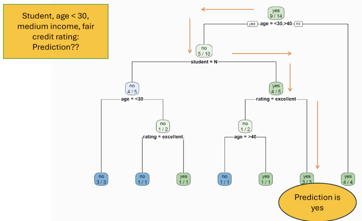
R produces this binary decision tree, and the red arrows represent the answer for the last row we’ve been looking for. What I see it did was to split every last leaf into a 100% certitude for each case.

And underfitted tree results in high bias and an overfitted tree results in high variance.

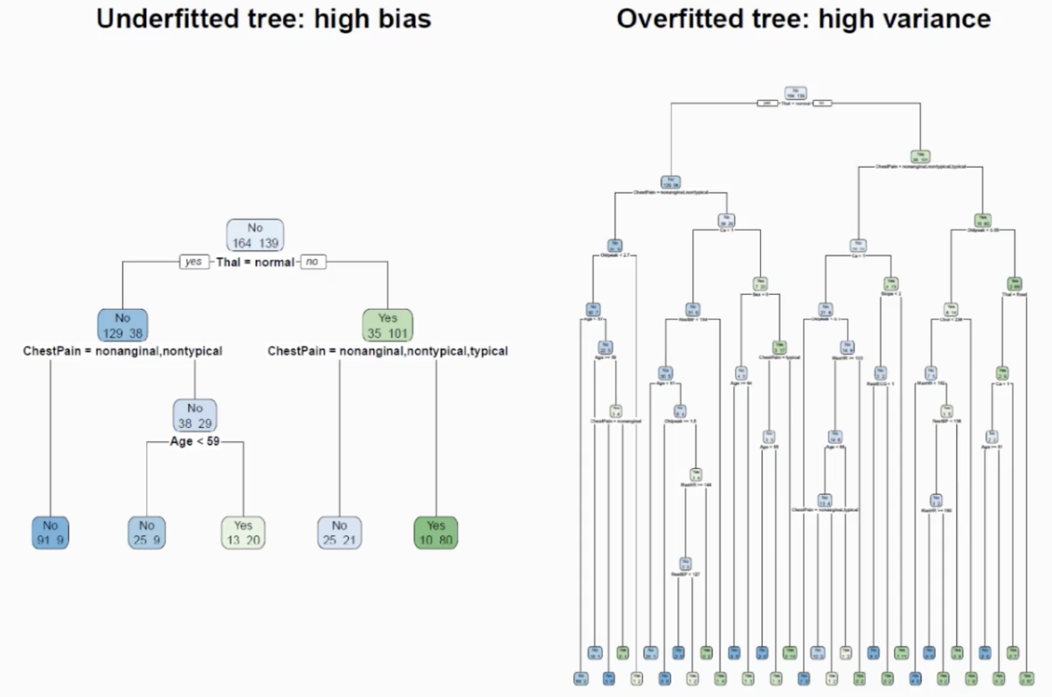
• the underfitted tree will not capture the underlying relationships in the data. It will perform poorly on both training and new data.
• the overfitted tree contains fits the training data extremely well. However, it is so complex that it also captures noise specific to the training dataset. As a result, its predictions will be much less accurate for new obsevations.
  • High variance means that small changes in the training data can lead to a very different tree.

Pruning Trees

The idea is to reduce the tree complexity in order to improve generalization and prevent overfitting.

We have two approaches:

1. Pre-pruning (early stopping)

• limit the maximum depth of the tree
• require a minimum amount of observations before a node may split
• require a minimum amount of observations in each leaf node

1. Post-pruning (prune after the tree has grown)

• grow full tree
• remove branches that do not improve predictive performance
• select the amount of pruning using cross-validation and the cost-complexity parameter.

Pre-pruning

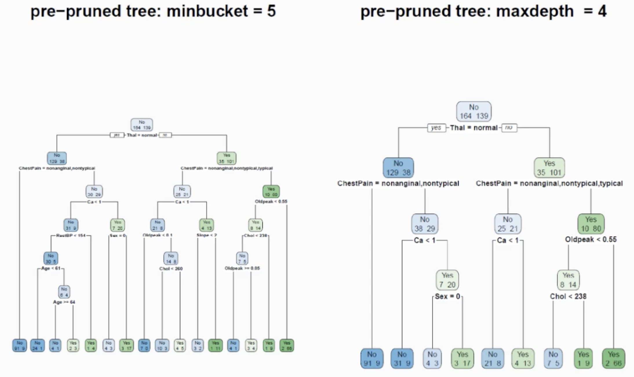
On the left, the minimum number of observations in each leaf node is set to 5. Therefore, if we have fewer than 5 observations, the algorithm does not split that branch.

On the right, the maximum tree depth is set to 4, meaning that no branch is allowed to extend more than four levels below the root node.

• In both cases, the complexity of the tree is reduced by stopping the growth of the tree early and it helps to reduce the risk of overfitting.

Post-pruning

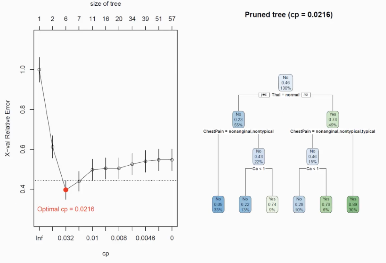
The algorithm first grows a large decision tree. From this tree, a sequence of increasingly simpler subtrees can be obtained by removing branches. The predictive performance of these trees is then estimated using cross-validation.

After computing the optimal cost parameter $cp$, we select the value of $cp$ that gives the lowest estimated prediction error (left graph). This value is then used to prune the original tree, resulting in the tree shown on the right.

The same idea can also be used for regression (continuous data). The difference is in how we measure similarity: instead of using the gini index, the algorithm chooses the split that gives the largest reduction in the within-node sum of squared errors (i.e. the splits are chosen typically based on the sum of squared errors). Once the tree is built, the predictions for a new observation is simply the mean outcome of the observations in the leaf (average).

Summary on Decision Trees

Strengths

• Fast to train, easy to understand and interpret
• Handles categorical and continuous predictors
• little data preprocessing required

Weaknesses

• can easily overfit without pruning
• sensitive to changes in the training data (high variance)
• often less accurate than ensemble methods such as Random Forests or Gradient Boosting.