Image Processing and Computer Vision

Notes for my Image Processing and Computer Vision exam at the University of Twente. It’s also a good summary of the lectures. I didn’t feel like making separate pages for each subject. They also serve as exam notes.

Most of the terms I have already used in:

• SeaClear
• Bachelors Thesis
• Barcode Detection and Decoding and others on GitHub.

Lecture 2

Intensity Transformations

• Some function that takes as input the old pixel value and gives the new one.
• Mostly used for image enhancement

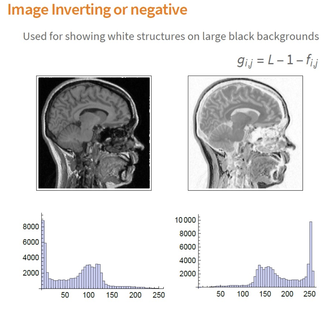
• Image inverting or negative: showing white structures on large black backgrounds.

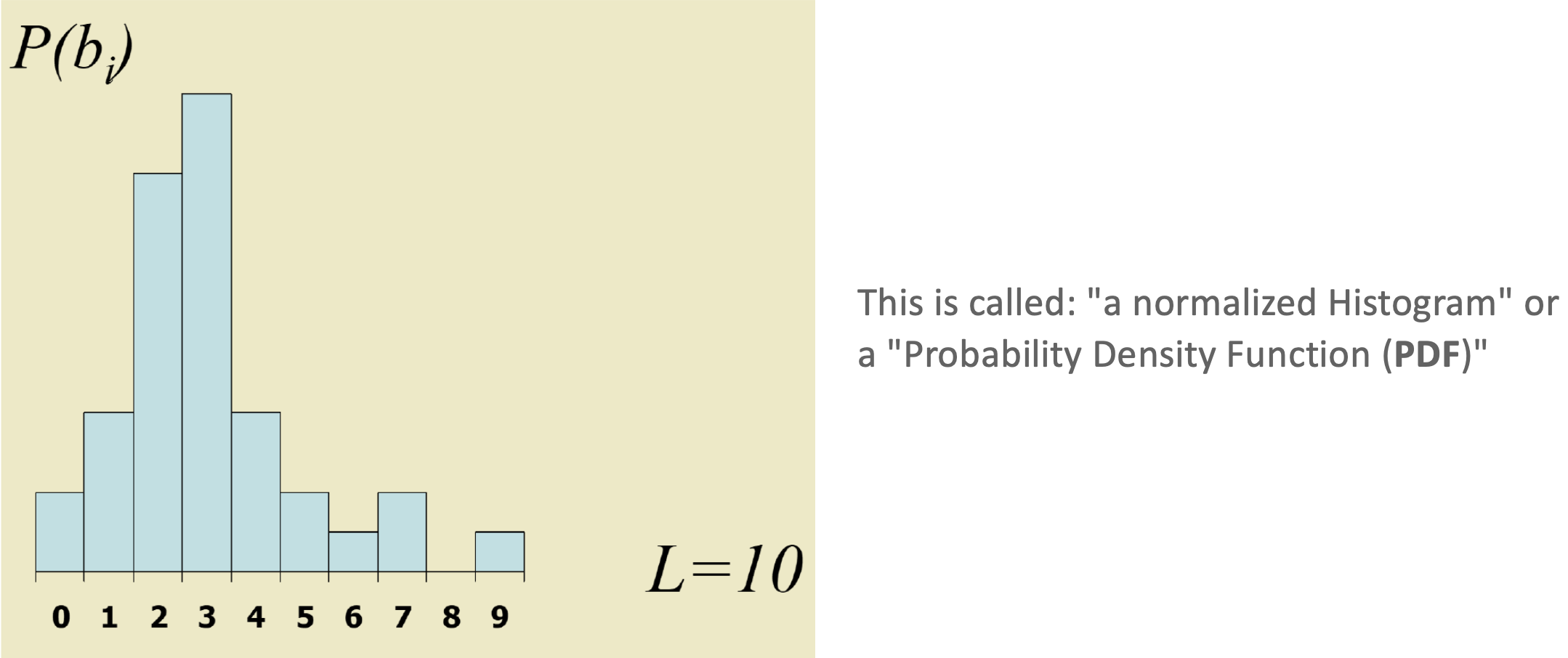
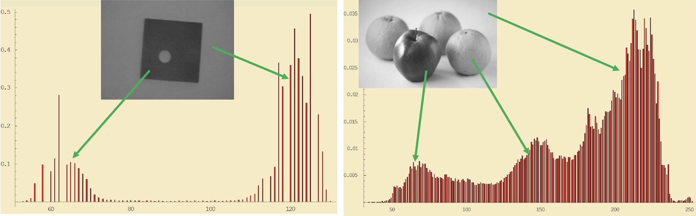
Histograms

As the teacher explained it, it’s basically a frequency vector of the intensity of vectors, divided by the total number of pixels.

• A histogram consists of bins $b_i$, with $i\in \{0,1,2,...,L\}$
• $N(b_i)$ = $\frac{N{o}_{pixels}}{voxels}$ for which $f(x)=b_i$
• $N$ is the total number of pixels. Then $P(b_i)=\frac{N(b_i)}{N}$

Gamma transformations

• $>=1$ means darker images
• $<1$ means brighter images

Color Spaces

• RGB (Red, Green, Blue)
• HSV (Hue, Saturation, Value)
• HSL (Hue, Saturation, Lightness)

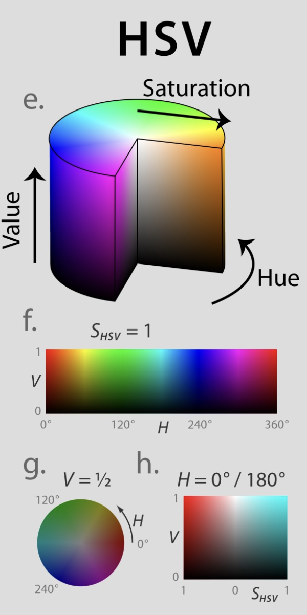
• Hue is the color of the image
• Saturation is the pureness of the Hue
• Value is the strength of the Hue

Image Filtering

Image Filtering

• in spatial domain, filtering is a mathematical operation on a grid of numbers (smoothing, sharpening)
• in frequency domain, filtering is a way of modifying the frequencies of images (denoising, sampling, compression)
• in templates and image pyramids, filtering is a way to match a template to the image (detection)

• Translating an image or multiplying/adding with a constant leaves the semantic context intact

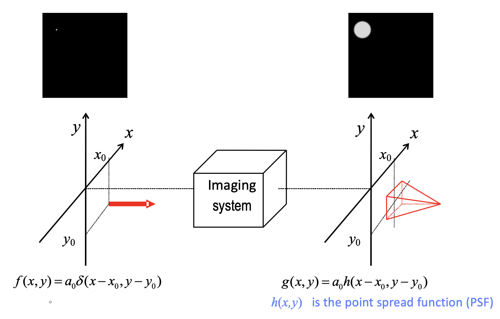
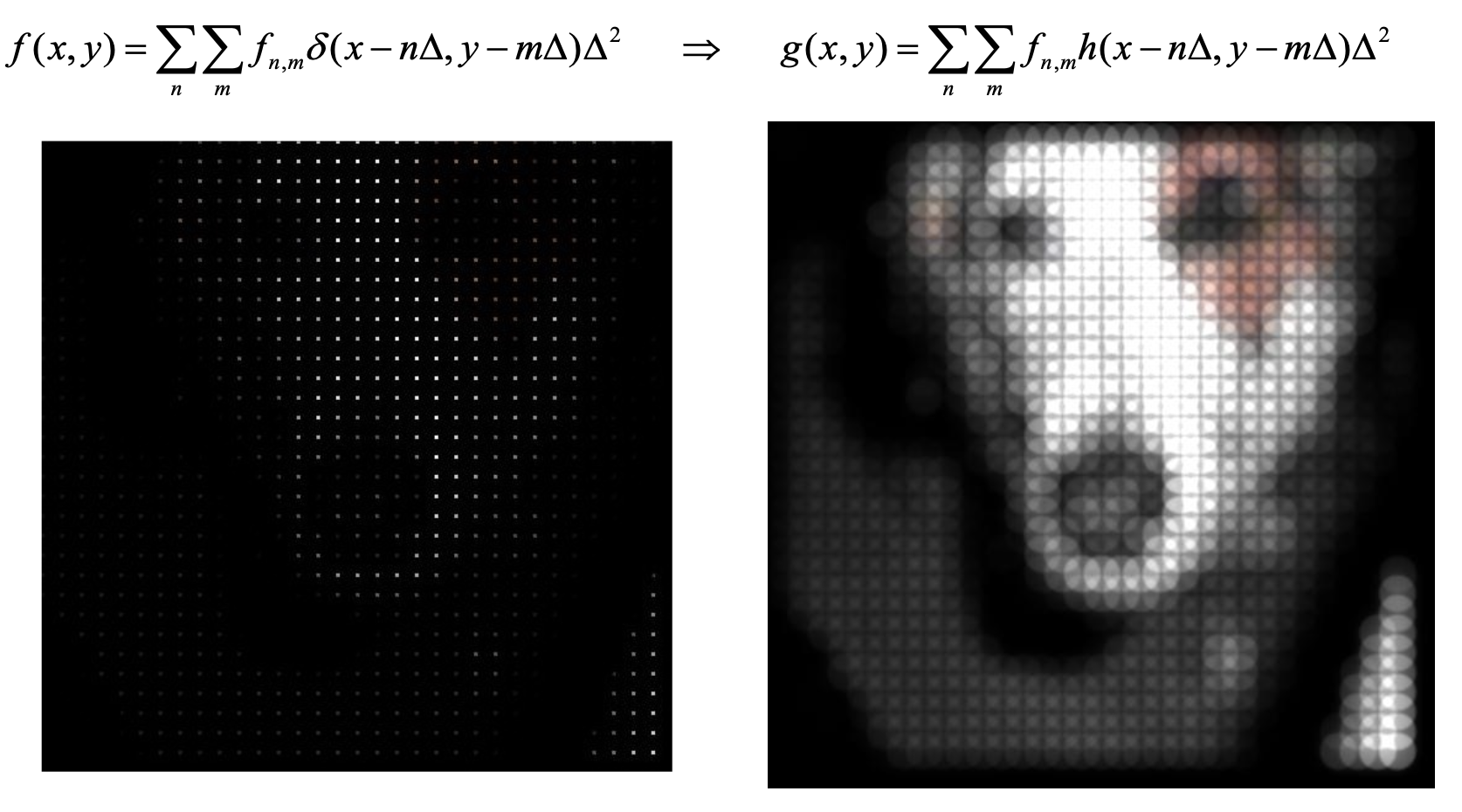
Intensity versus Point Spread Functions (PSF)

Convolution

• 2D: $g(x,y)=f(x,y)\ast h(x,y)$

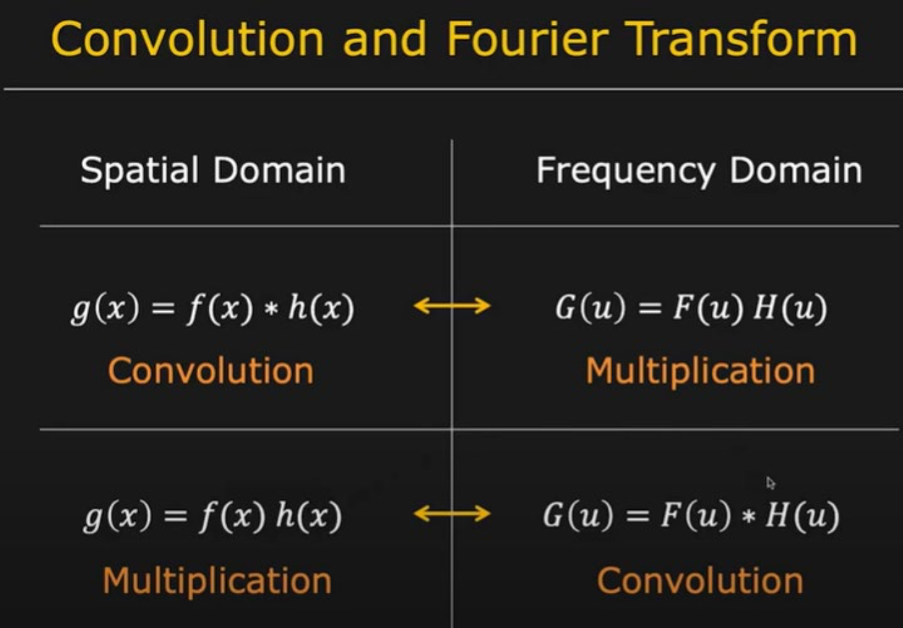
Convolution Theorem

• Convolution in space domain is equivalent to multiplication frequency domain

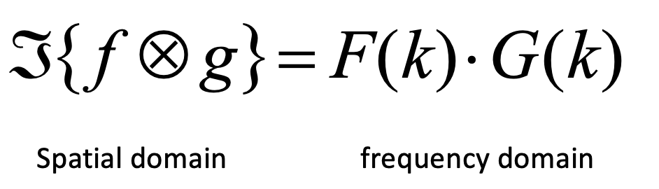
• After convolution, the resulting size is reduced $(n-k+1)$

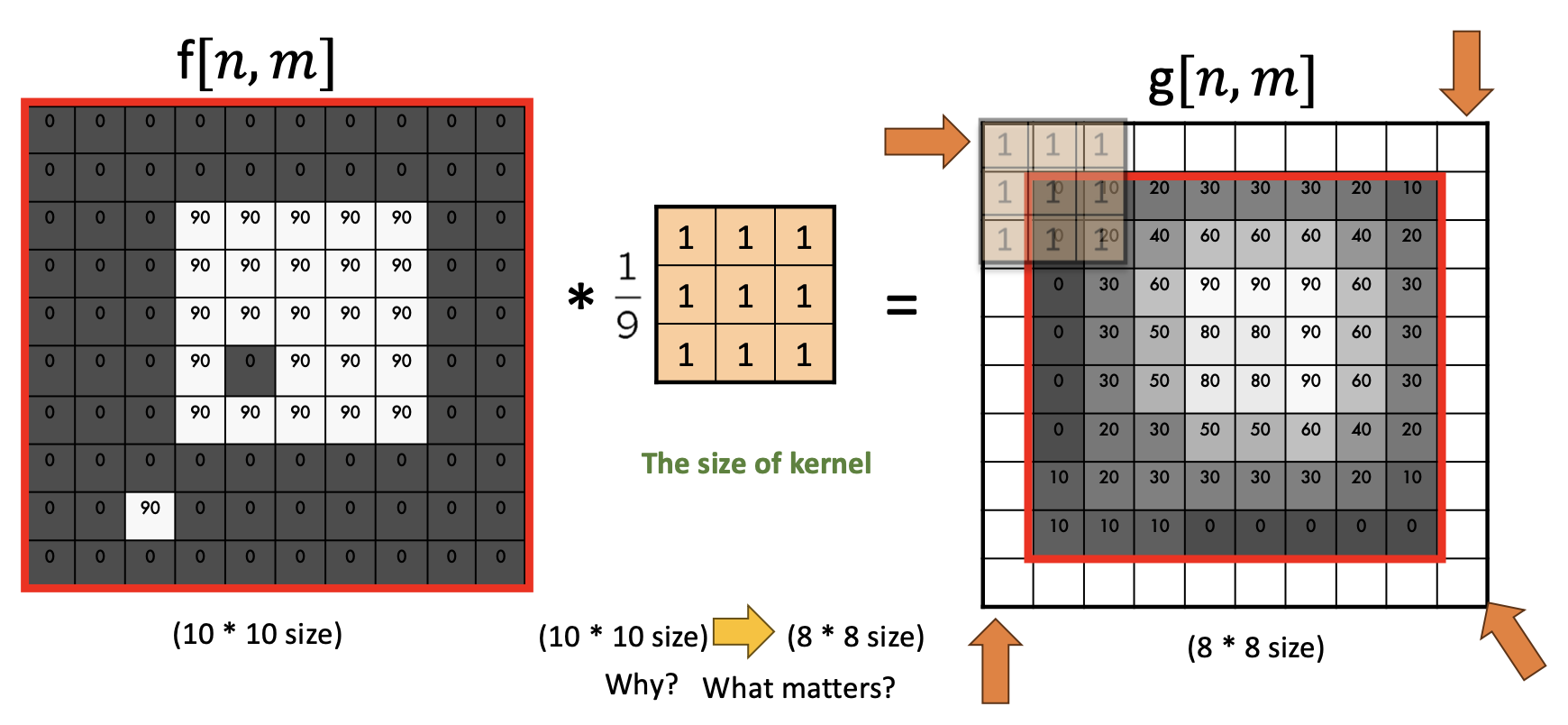
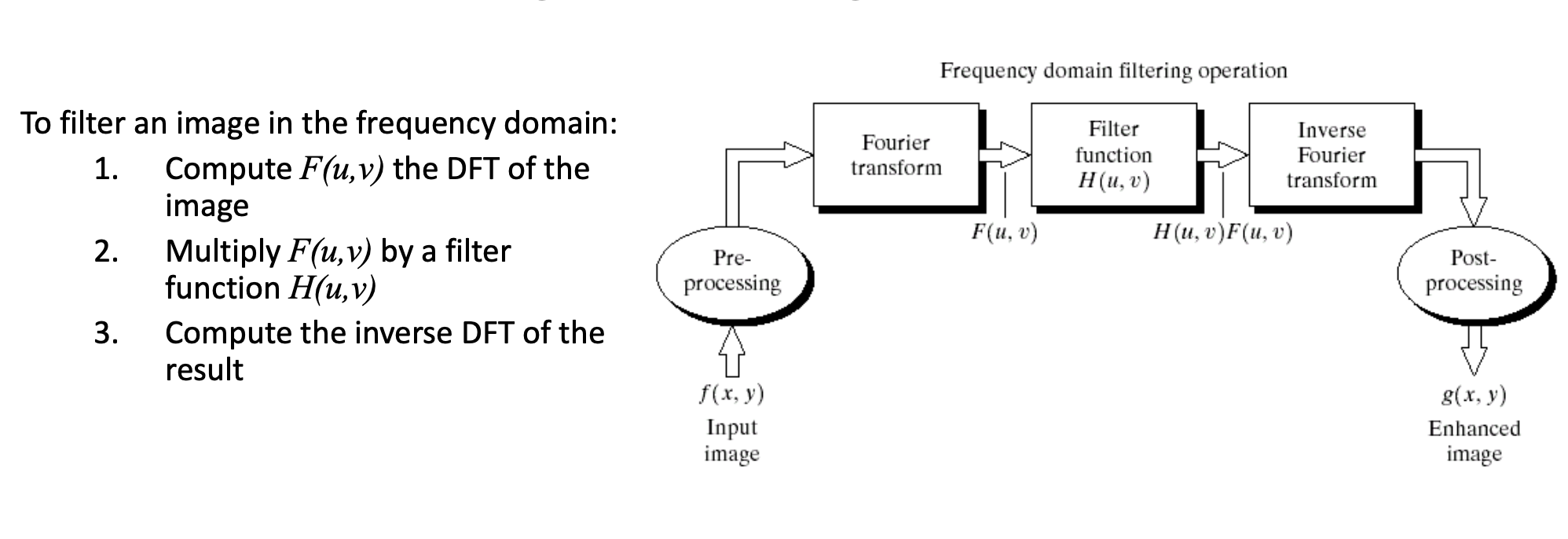
Image Restoration

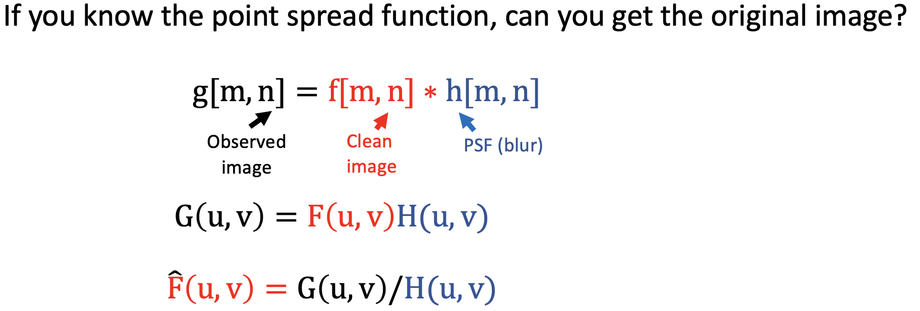
• Limit $\frac{1}{H(u,v)}$ to avoid 0 in the denominator!

Moving Average

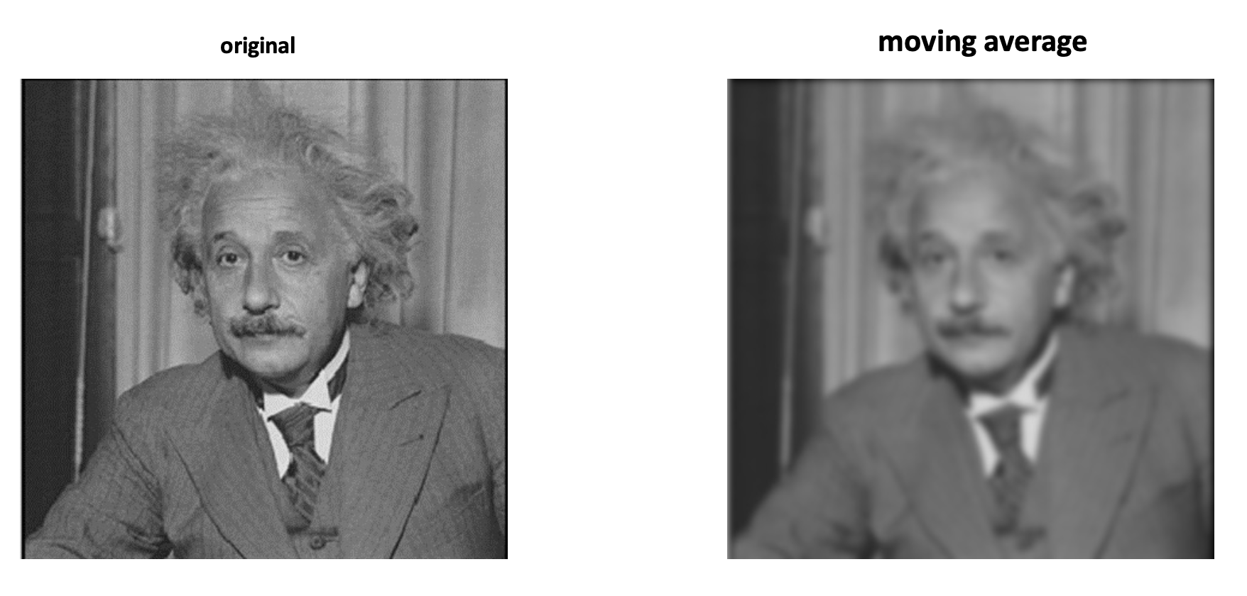
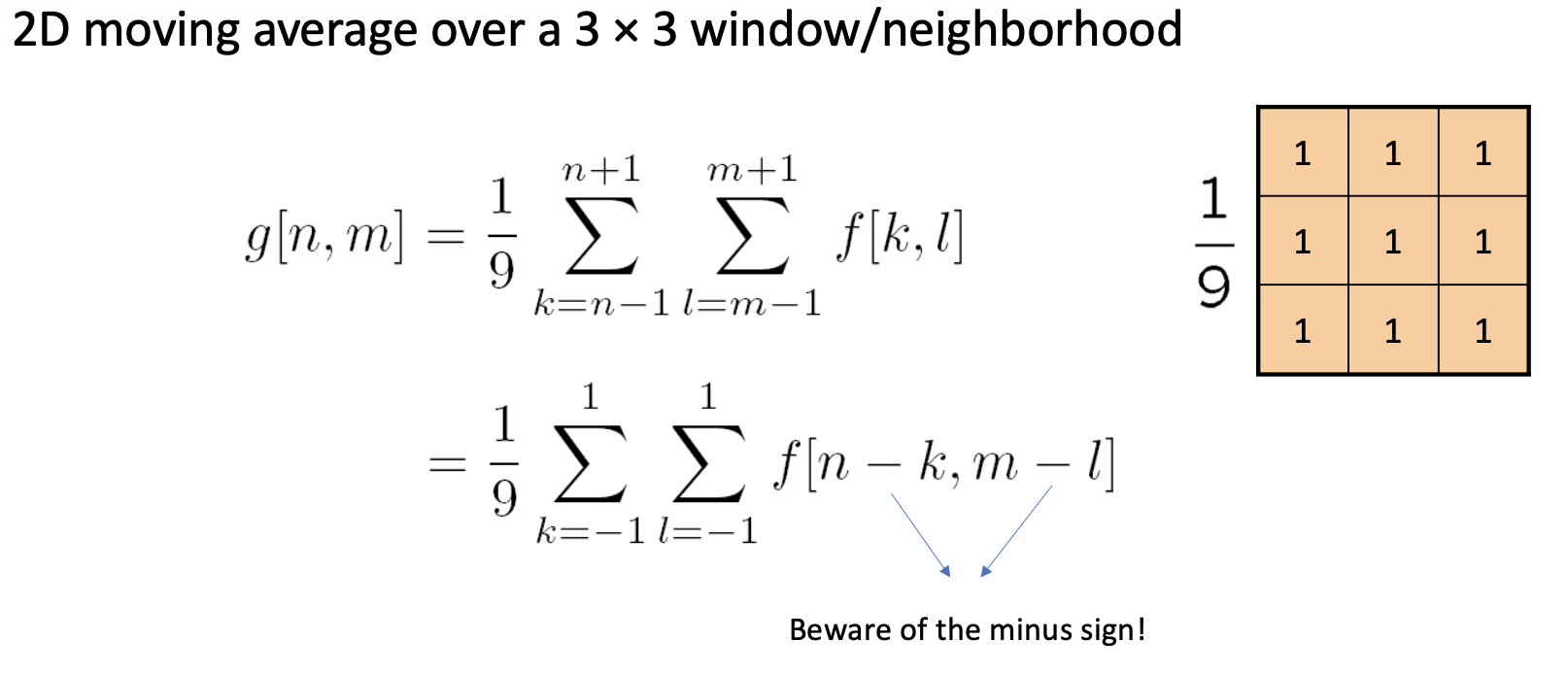
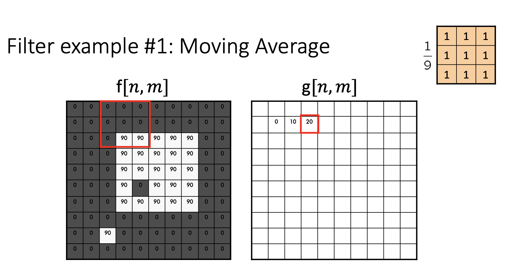
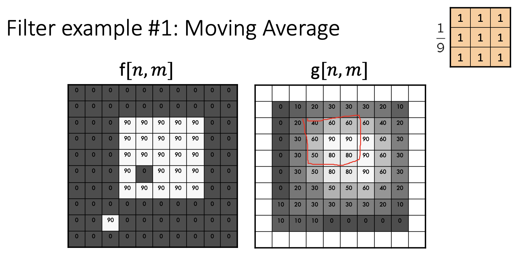
What this specific filter does:

• It smoothens the image
• It calculates the average in a $3\times 3$ neighborhood

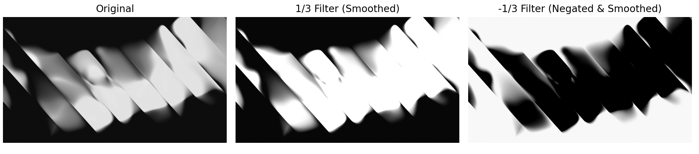
So if the kernel was $-\frac{1}{9}$

The rule would be: Output = -(sum of 9 neighboring pixels) / 9 = -average

• The result would be the inverse of the above one. So bright regions become darker and dark regions become brighter.

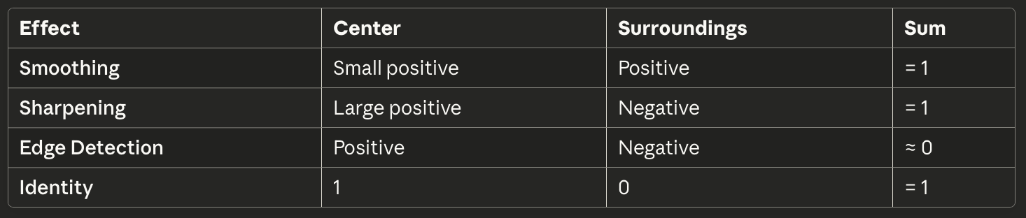
Some rules of thumb for each operation

A kernel does

• Darkening — sum of all elements < 1
• Brightening — sum of all elements > 1
• Smoothing — positive weights distributed
• Sharpening — when the center value is large and positive, the surrounding values are negative and the sum == 1.

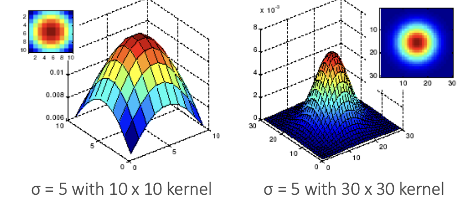
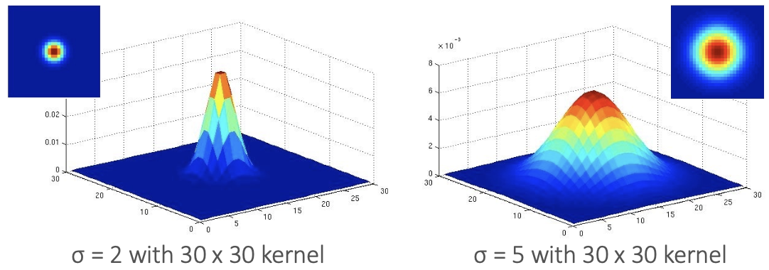
Gaussian Filter

• Smoothing
• Denoising

Key Parameters

1. $\sigma$ (sigma/variance): controls blur strength (extent of smoothing)

• Small $\sigma$ (e.g. 2) = sharp, concentrated, less blur

• Large $\sigma$ (e.g. 5) = wide, spread-out, more blur

2. Kernel size: must be large enough to capture the Gaussian shape

• Too small: truncates the Gaussian bell curve

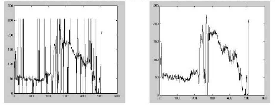
Non-linear Filters

Median Filter

• A median filter operates over a window by selecting the median intensity in the window
• Good for salt-and-pepper noise
• Robustness to outliers (in comparison with Gaussian)
• Edge-preserving (in comparison with Gaussian)

Correlation vs Convolution

• In convolution, we flip the kernel
• A convolution is an integral that expresses the amount of overlap of one function as it is shifted over another function. (filtering operation)
• Correlation compares the similarity of two sets of data. Correlation computes a measure of similarity of two input signals as they are shifted by one another. The correlation result reaches a maximum at the time when the two signals match best (measure of relatedness of two signals)

Template Matching

• It’s done through Normalized cross-correlation

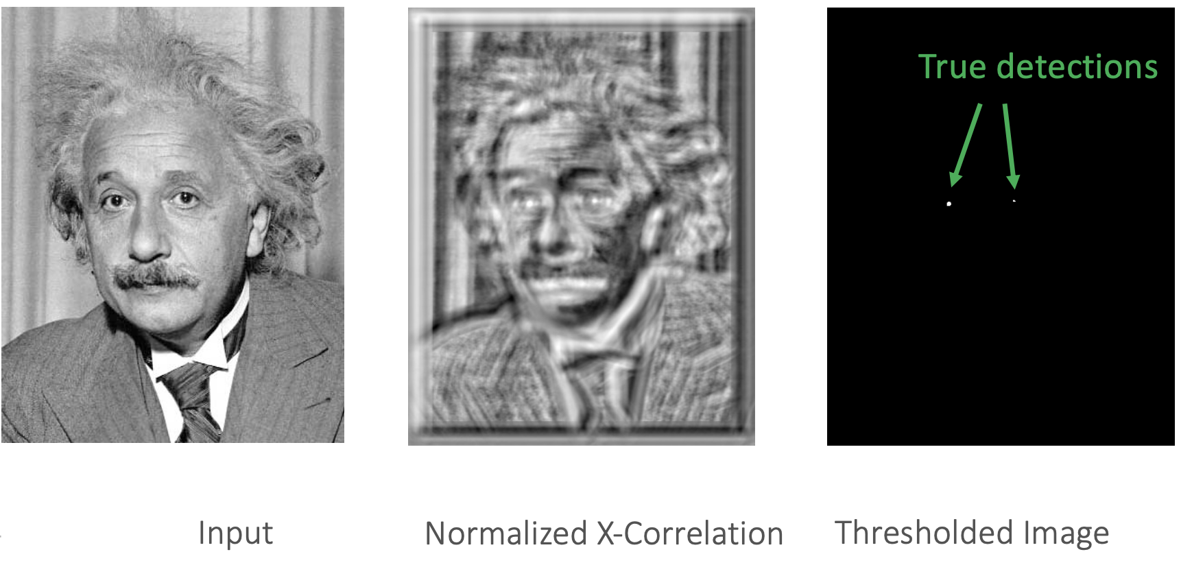
• Matching depends on
  • scale,
  • orientation,
  • general appearance

Lecture 3 — Fourier Transform and Convolution

Fourier Transform

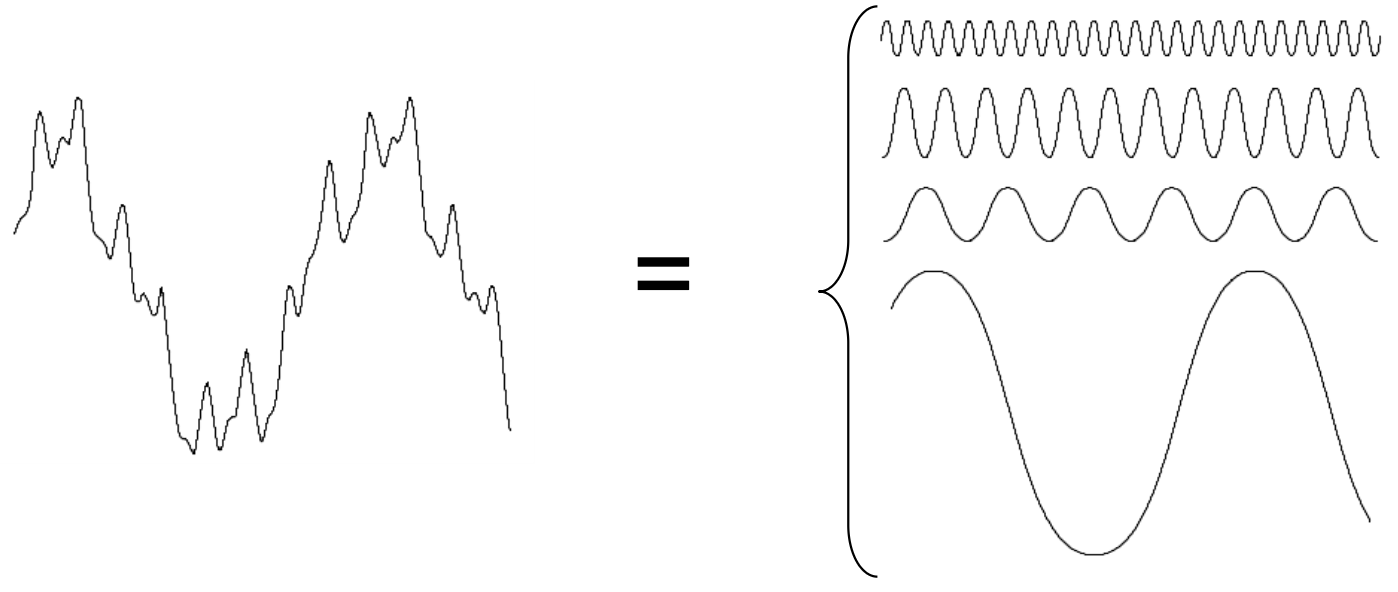
Fourier Theory

Any function that periodically repeats itself can be expressed as a sum of sines and cosines of different frequencies each multiplied by a different coefficient – a Fourier series.

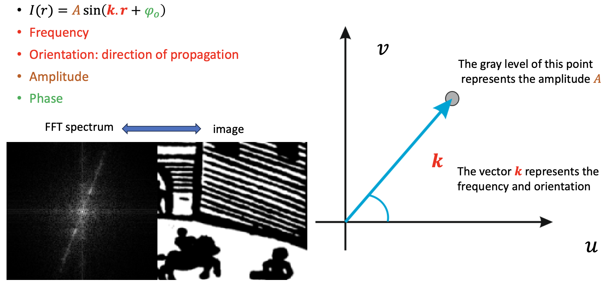
Important parameters

• Frequency: $sin(kx)\to k$
• Amplitude: $A\cdot sin(kx)\to A$
• Phase: $A\cdot sin(kx+{\theta }_0)\to {\theta }_0$
• Orientation: $I(r)=A\cdot sin(k.r+{\theta }_0)$

Spectrum

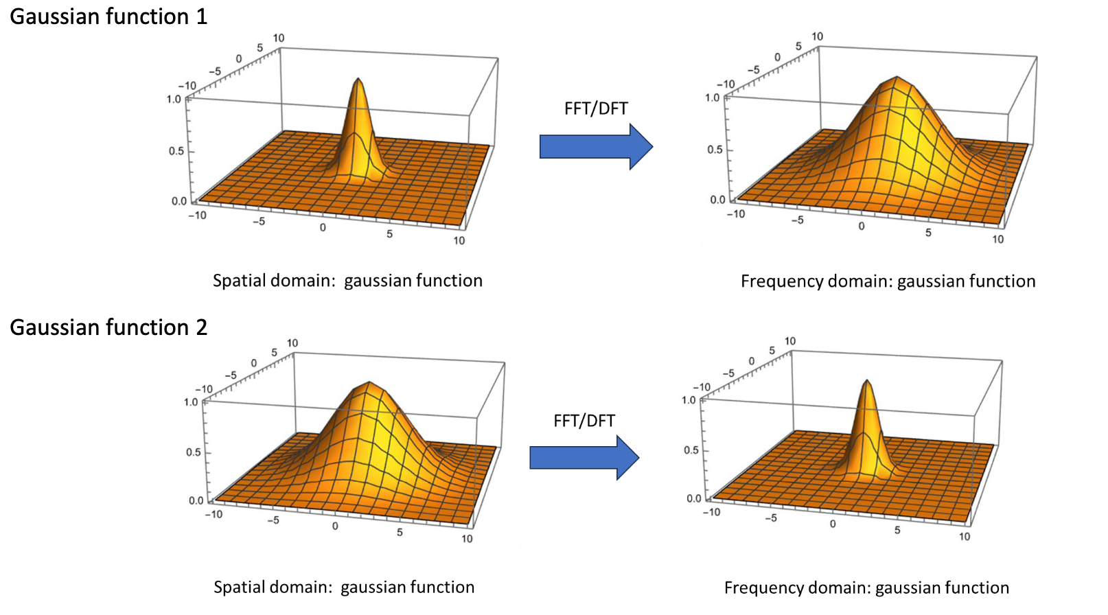
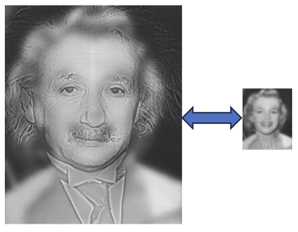
Fourier Uncertainty Principle

Narrow in Space $\to$ Wide in Frequency

• Spatial Domain: The function is a narrow spike. This means the signal is highly localized in space (it exists intensely at one small spot, around (0,0), and is zero almost everywhere else).
• Frequency Domain: The resulting function is wide and spread out. To create such a sharp, sudden spike in the spatial domain, you need to combine many different frequencies (both low and high). This “wide-band” combination of frequencies results in a wide, spread-out plot in the frequency domain.

Wide in Space $\to$ Narrow in Frequency

• Spatial Domain: The function is a wide, broad hill. This means the signal is delocalized (spread out) in space. It changes very smoothly and gradually.
• Frequency Domain: The resulting function is a narrow spike. Because the spatial function is so smooth and changes slowly, it is composed almost entirely of low frequencies. It doesn’t need high frequencies (which create sharp changes). This “narrow-band” signal is highly localized around the zero-frequency (DC) component, resulting in a narrow spike.

So, in short:

• To localize a signal in space (make it narrow), you must delocalize it in frequency (make it wide).
• To localize a signal in frequency (make it narrow), you must delocalize it in space (make it wide).
• You can’t have a function that is “narrow” in both the spatial and frequency domains simultaneously.

Convolution Theorem

• Convolution in space domain is equivalent to multiplication frequency domain.
• Multiplication in space domain is equivalent to convolution in frequency domain

Gaussian Low-Pass Filter

• Used to connect broken text

Gaussian High-Pass Filter

• Image restoration

Lecture 4 — Morphological Operations

• Morphological Operations are based on set theory (inclusion, union, difference, etc.)

Neighborhoods and Adjacents

• two pixels $a$ and $b$ are:
  • 4-connected if $b\in N_4(a)$
  • 8-connected if $b\in N_8(a)$

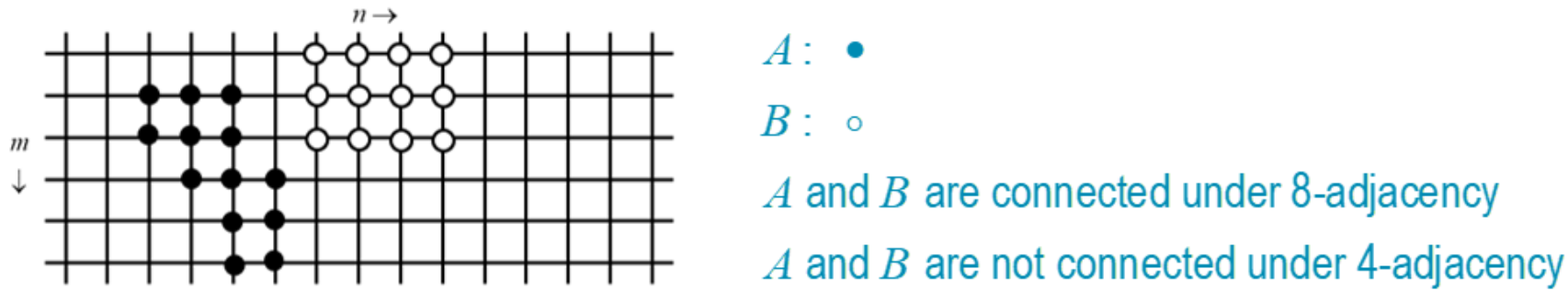
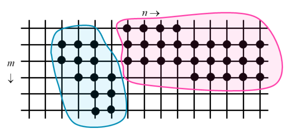
• Two pixels $a$ and $b$ are connected in region A if a path exists between $a$ and $b$ entirely contained in $A$.

• The connected components of $A$ are the subsets of $A$ in which:

  • all pixels are connected in $A$,
  • all pixels in $A$ not belonging to the subset are not connected to that subset.

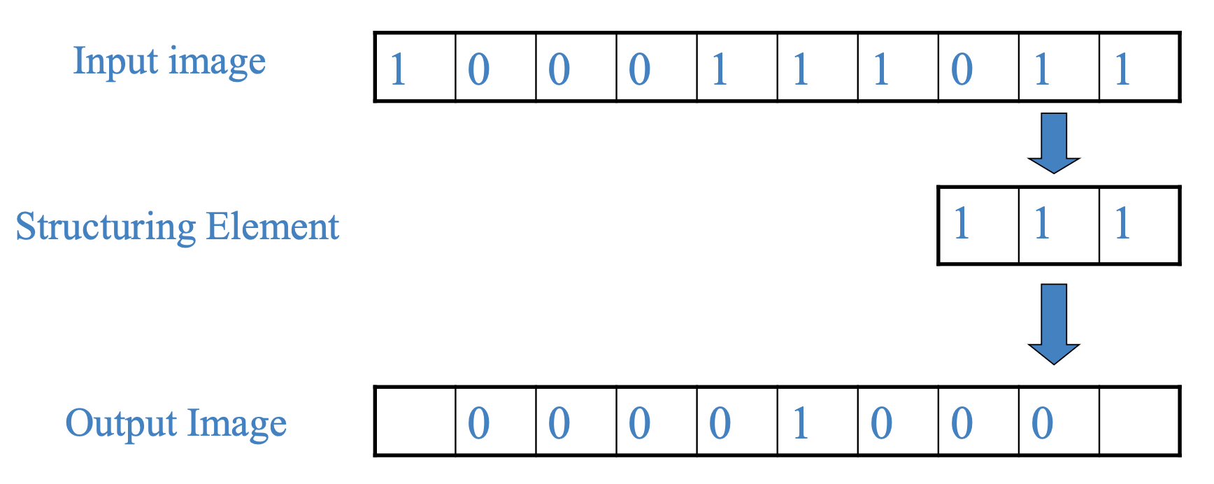
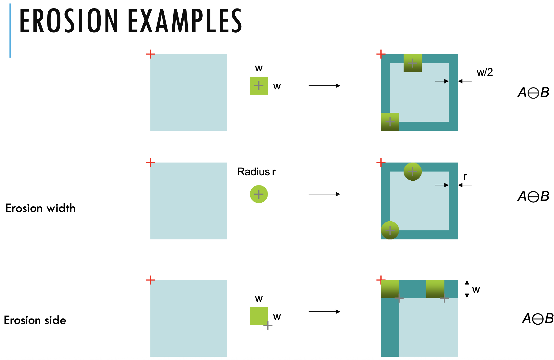
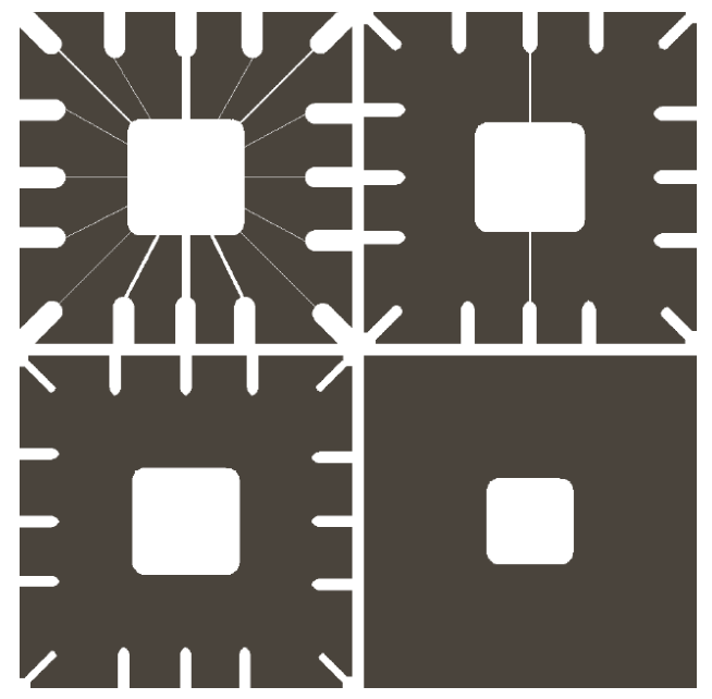
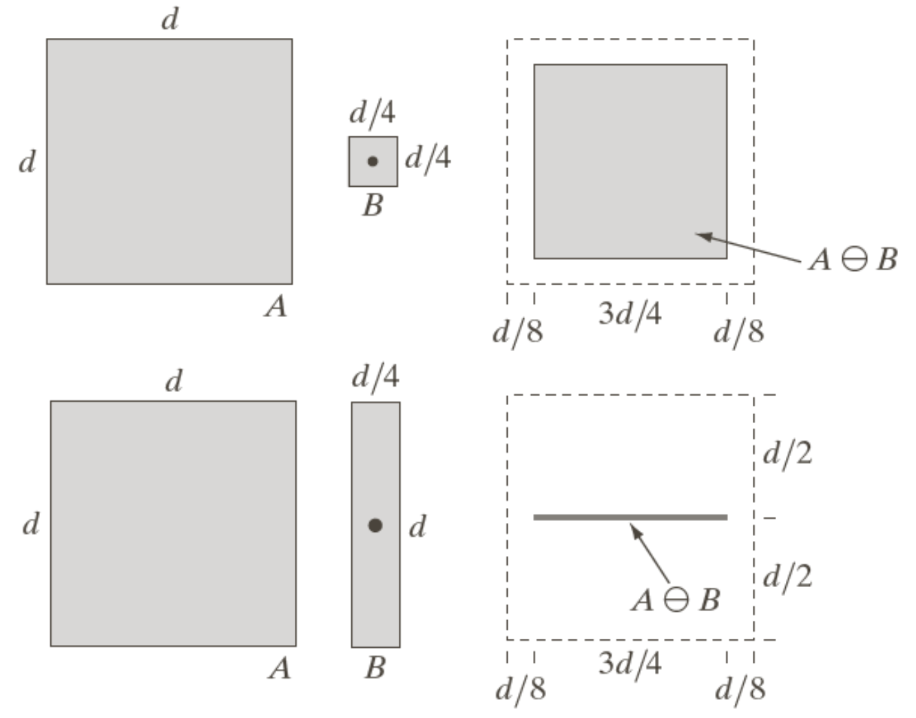
Erosion

Erosion

• Enlarges holes,
• Breaks thin parts,
• shrinks objects
• is not commutative
• Match completely
• $A\ominus B$

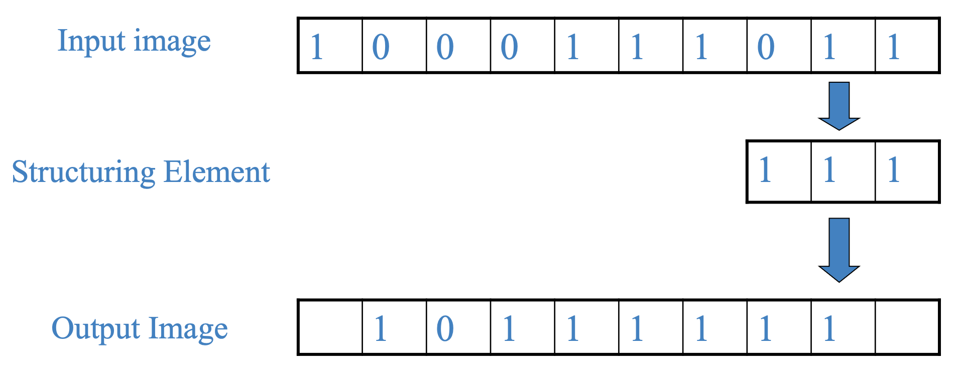
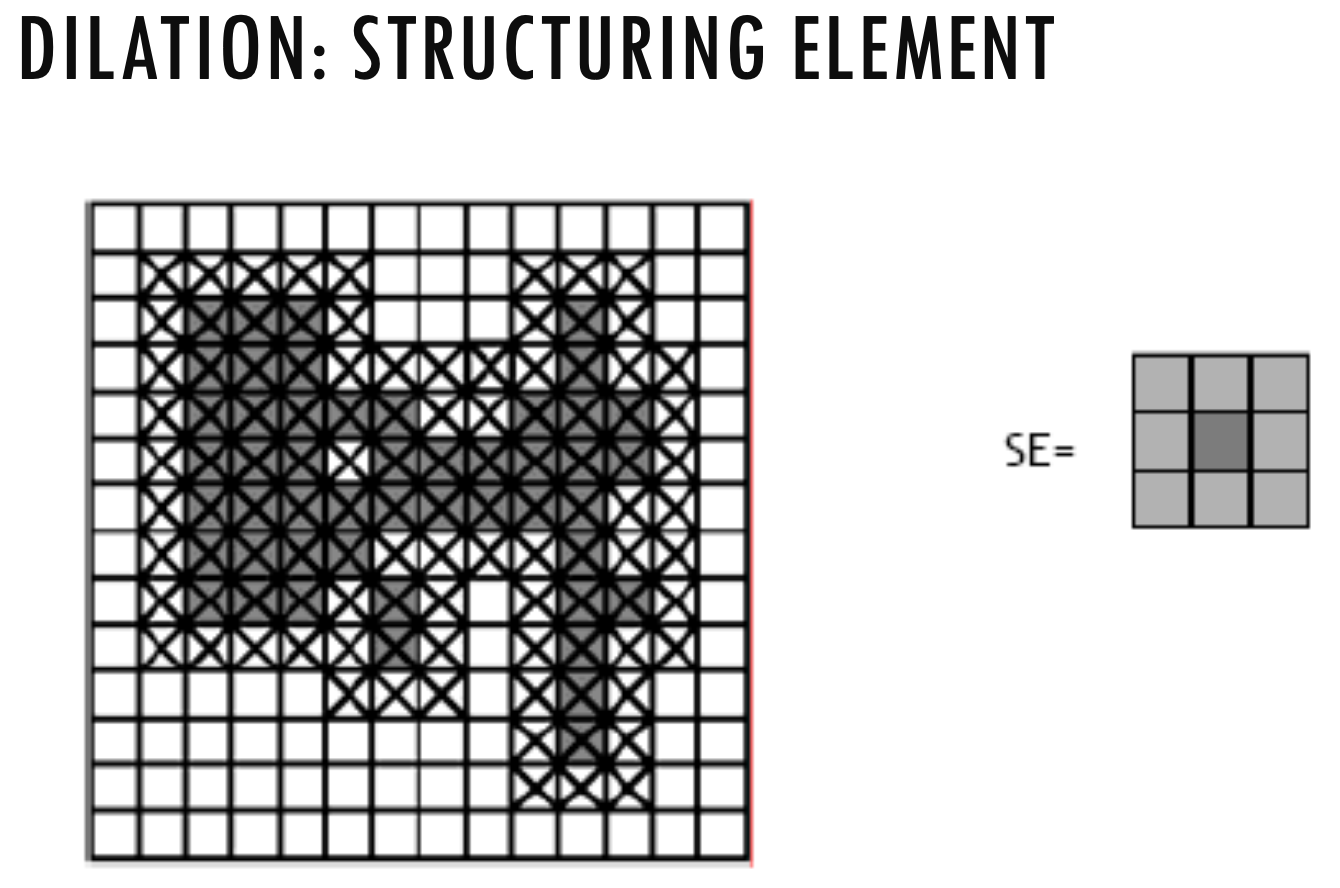
Dilation

Dilation

• Filling of holes of certain shape and size
• Match at least one element
• $A\oplus B$

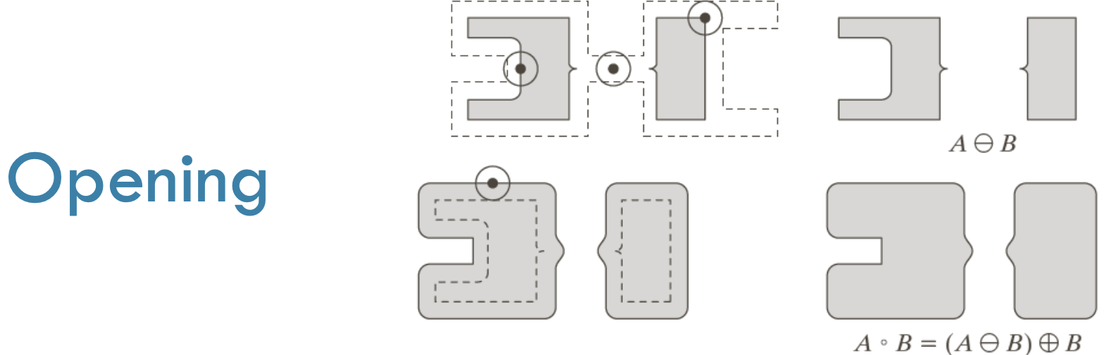
Opening

• $A\cdot B=(A\ominus B)\oplus B$
• erosion, then dilation

Hit or Miss

• Find location of one shape among a set of shapes ”template matching”
• Shape recognition

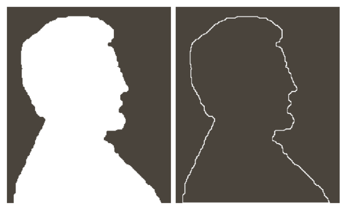
Boundary Extraction

• We can simply do $A-(A\ominus B)$

Lecture 5: Scale Space, Image Derivative and Edge Detection

• By changing the zoom-in/out ratio, we can see the different levels of information from the image.

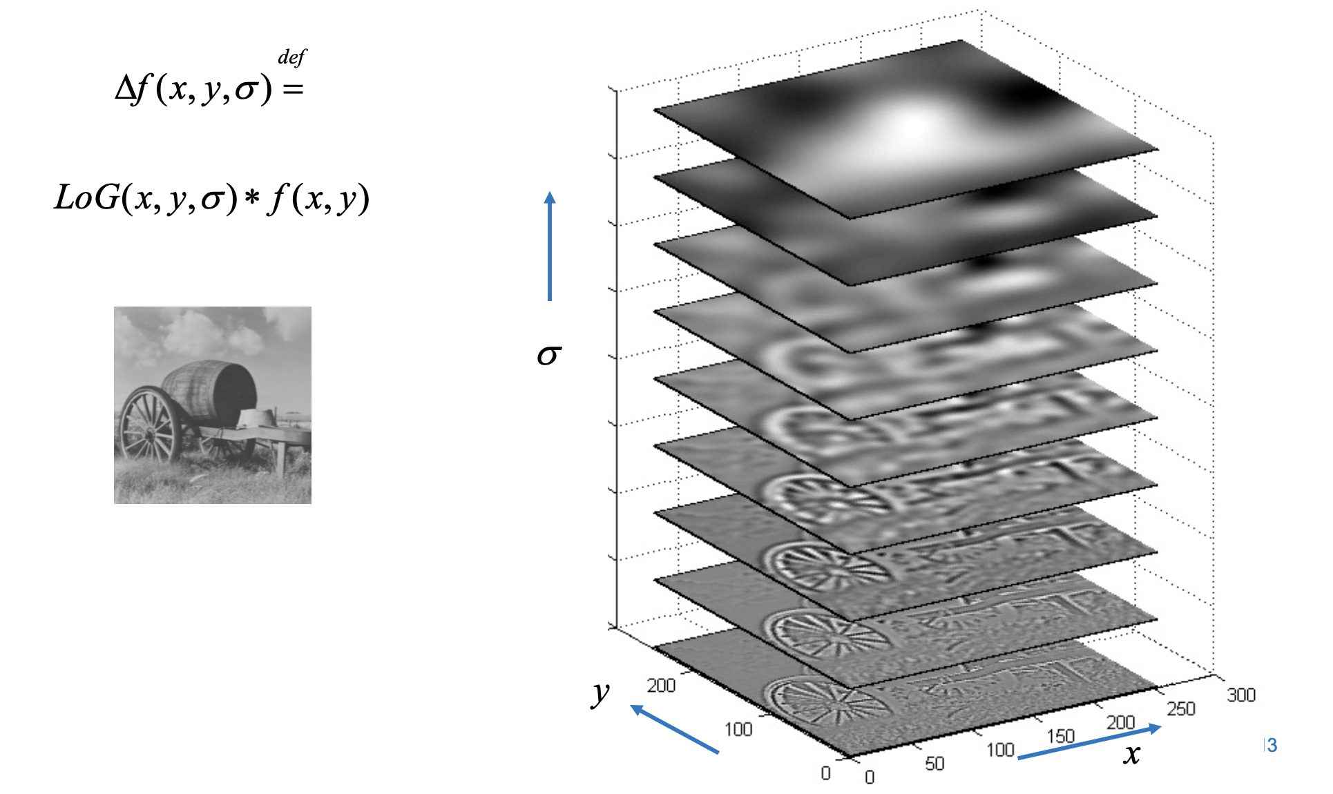
Scale Space Theory: Convolution with Gaussian

• The PSF of the operation is a Gaussian:
  • $h(x,y,{\sigma }^2)=\frac{1}{2\pi {\sigma }^2}\exp \left(-\frac{x^2+y^2}{2{\sigma }^2}\right)$
  • scale is parametrized by ${\sigma }^2$

Properties of Convolution

1. Commutativity: $f(x,y)\ast h(x,y)=h(x,y)\ast f(x,y)$
2. Associativity: $(f(x,y)\ast h(x,y))\ast g(x,y)=f(x,y)\ast (h(x,y)\ast g(x,y))$

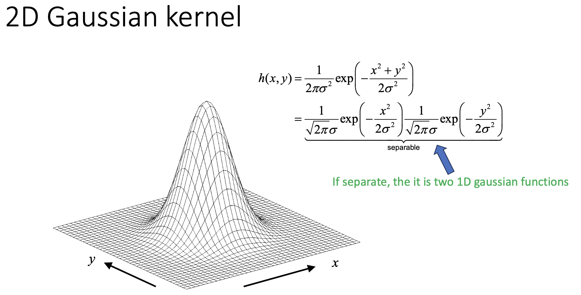
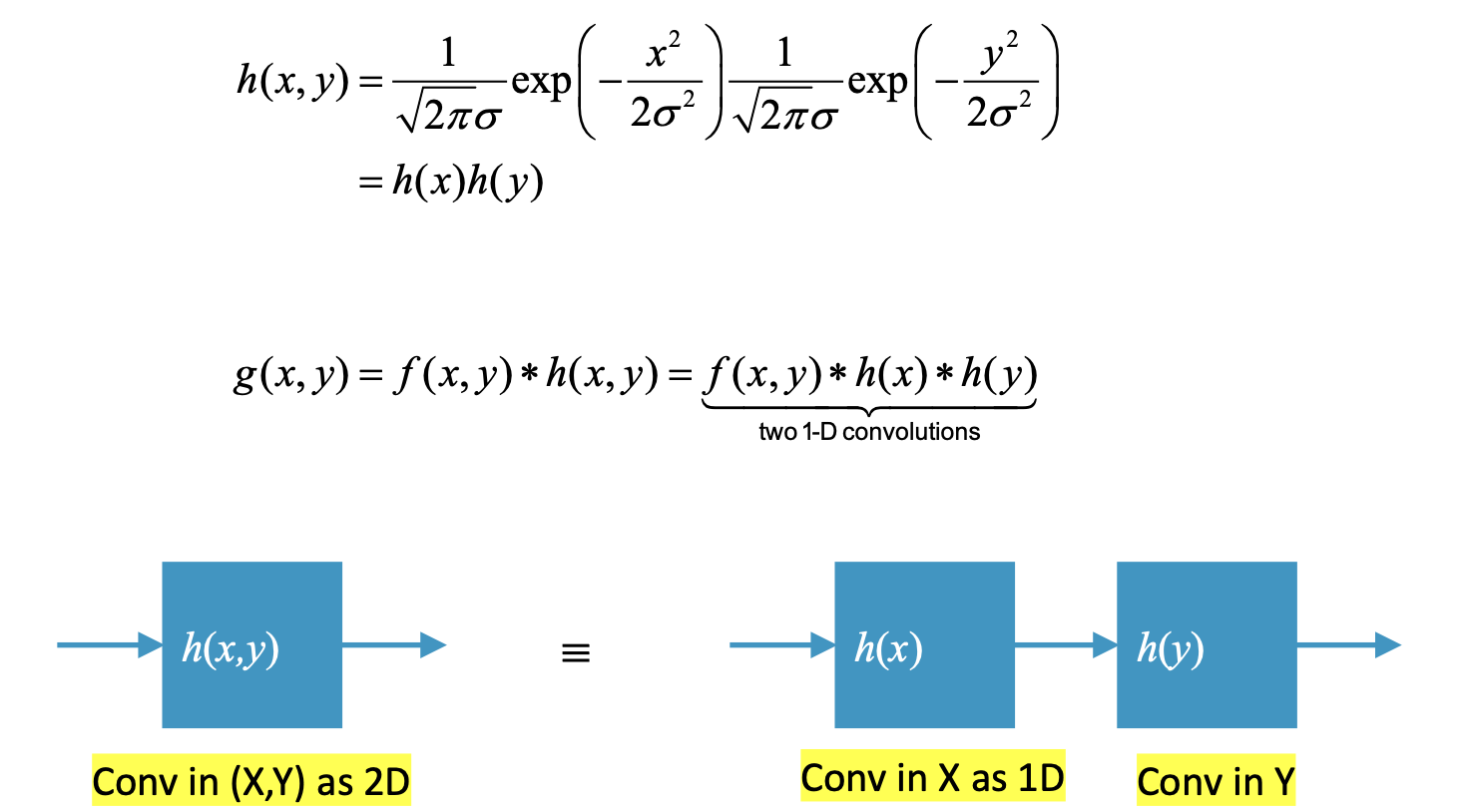
Properties of Gaussian Functions

1. Separability property: The Gaussian is the only PSF that satisfies

   • $h(x,y,a)\ast h(x,y,b)\equiv h(x,y,a+b)$
   • This means convolving with two Gaussians sequentially is equivalent to convolving with a single Gaussian whose variance is the sum.

2. Fourier transform property:

   • Spatial domain: $h(x,y,{\sigma }^2)=\frac{1}{2\pi {\sigma }^2}exp(-\frac{x^2+y^2}{2{\sigma }^2})$
   • Frequency domain: $H(u,v,{\sigma }^2)=exp(-2{\pi }^2{\sigma }^2(u^2+v^2))$

3. Convolution in Fourier Domain:

   • $h(x,y,{\sigma }_1^2)\ast h(x,y,{\sigma }_2^2)=h(x,y,{\sigma }_1^2+{\sigma }_2^2)$
   • The only PSF that satisfies this is a Gaussian

An increase of scale

• blurs the image,
• gives rise to less structure,
• decreases noise

Scale space applications: SIFT

Key applications of scale space:

• Edge and blob detection,
• Feature extraction (e.g., SIFT, SURF),
• Object recognition and tracking.

Gaussian Convolution, Image Derivative

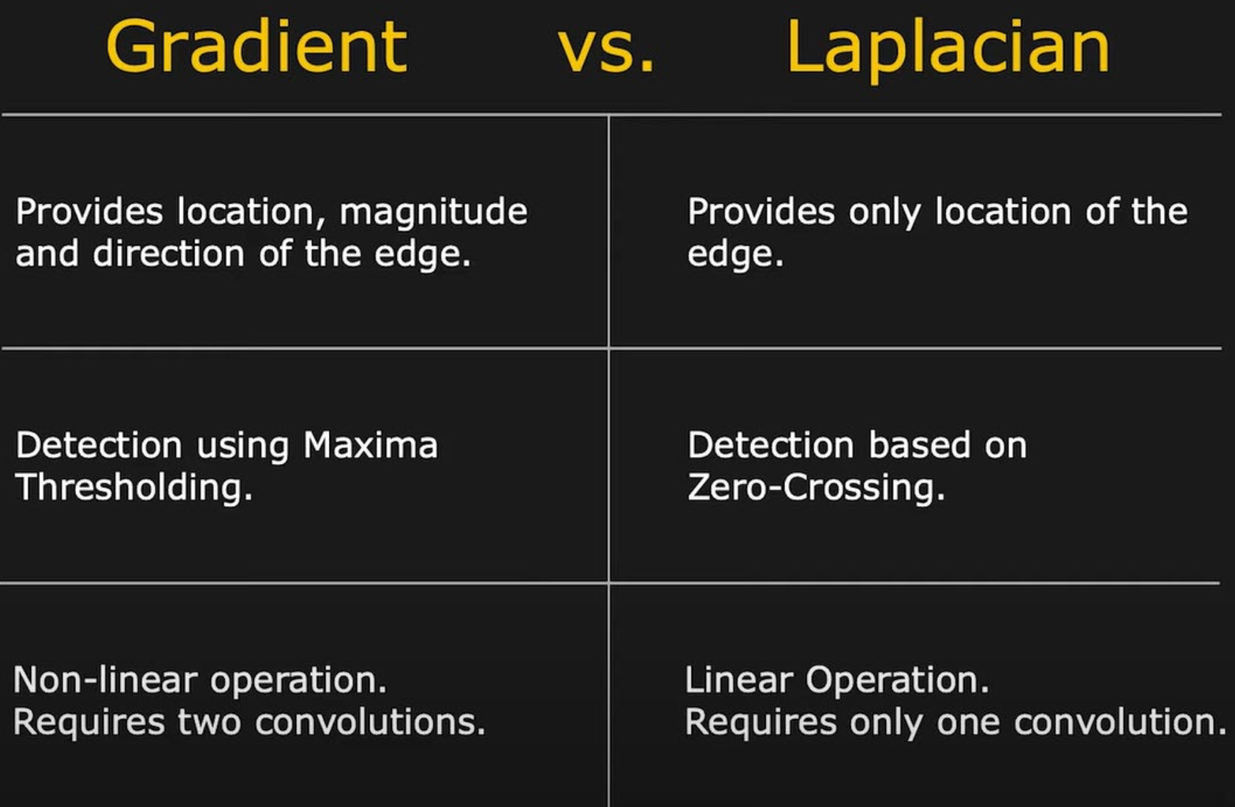
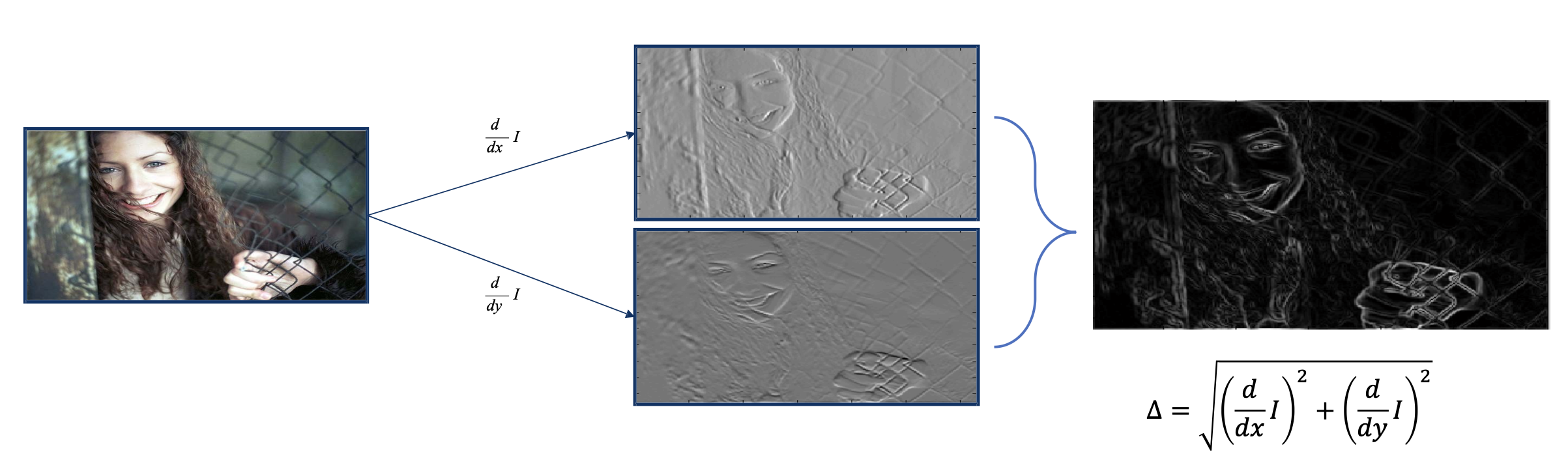
Gradient Vector

• Is in the direction of change in intensity (perpendicular to the contour lines),
• Towards the direction of the higher intensity.

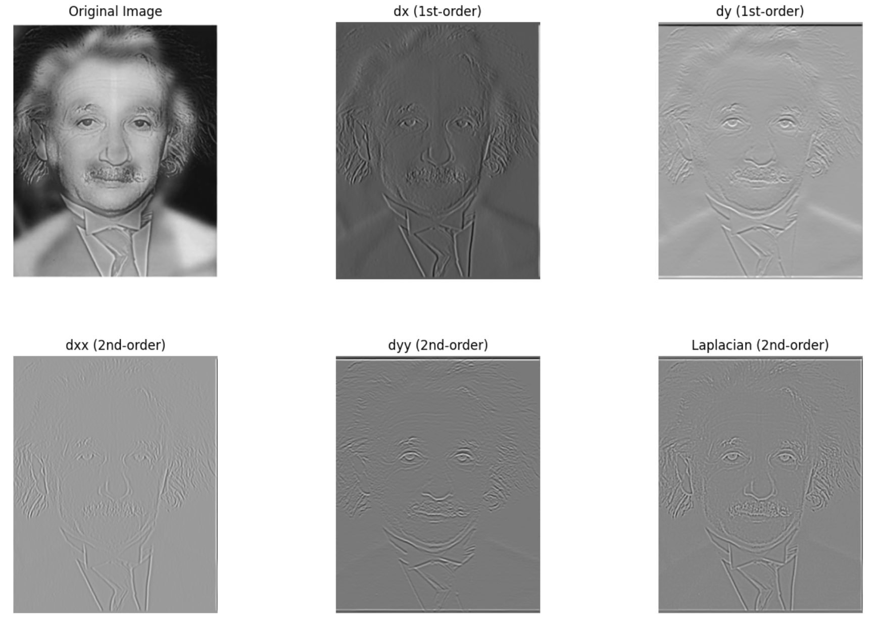
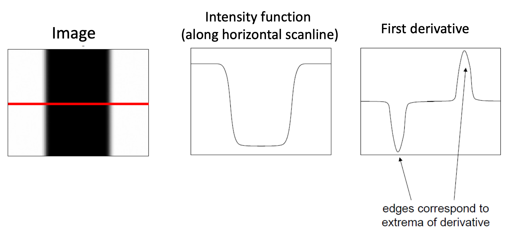
First Derivatives

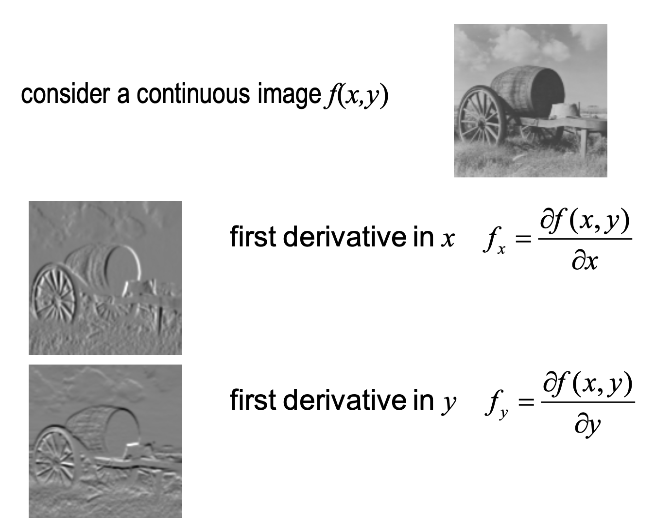
• Gradient Magnitude: $\sqrt{f_x^2+f_y^2}$
• Gradient Argument: $arctan(\frac{f_y}{f_x})$
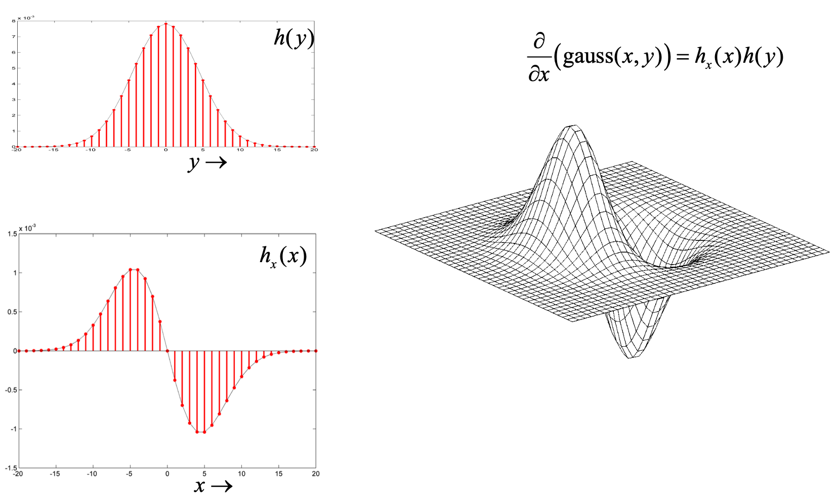
• First derivative in x direction is convolution with derivative of Gaussian== $f_x(\sigma )=f\ast h_x(\sigma )$
• Same for second derivative in y direction $f_{yy}(\sigma )=f\ast h_{yy}(\sigma )$

Second Derivatives

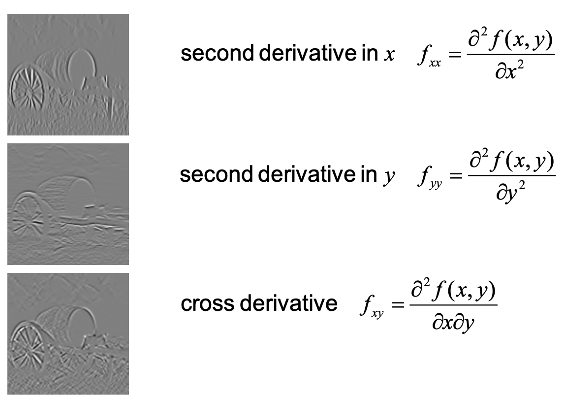
Laplacian

• $△f(\sigma )=f\ast △h(\sigma )$
• $△h(\sigma )=h_{xx}(\sigma )+h_{yy}(\sigma )$
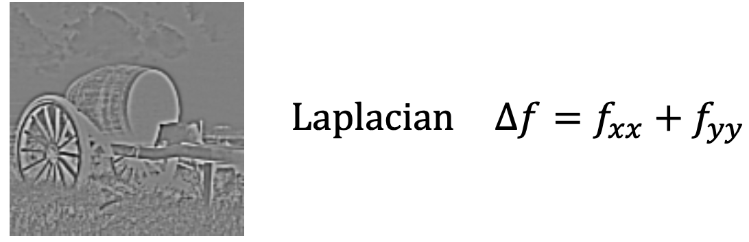
• Laplacian Zero-Crossing: all locations where $△f(\sigma )$ are zero
• $△f(x,y,\sigma )=LoG(x,y,\sigma )\ast f(x,y)$

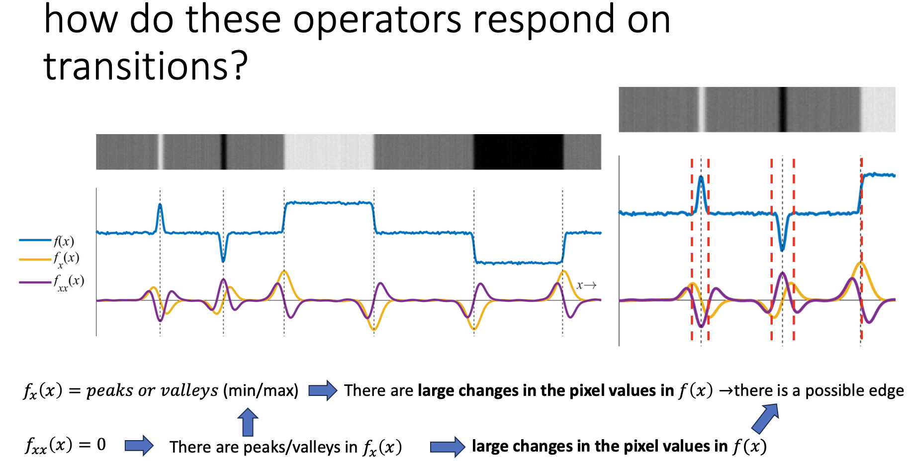
1D Edge Detection

$f(x)=ϵ\cdot step(x-x_0)+noise(x)$

• $ϵ=0$ no edge
• $ϵ=1$ edge

2D Edge Detection

• An edge is a place of rapid change in the image intensity function

• Affected by noise

Derivative Theorem of Convolution

• $\frac{d}{dx}(f\ast g)=f\ast \frac{d}{dx}g$
• $f$ is the image
• $g$ is the convolution kernel

To calculate image derivative:

1. You do the corresponding derivative on the convolution kernel (= Gaussian)
2. You used the result of (1) to do the convolution with your image

• As $\sigma$ increases,
  • more pixels are involved in average
  • image is more blurred
  • noise is more effectively suppressed

Edge Detectors

Steps

1. Compute derivatives in x and y directions
2. Find gradient magnitude
3. Threshold gradient magnitude ⇒ edges

How does Sobel differ from Prewitt?

• Adds extra weight (2) to the central row/column.
• introduces a smoothing effect (weighted average), making Sobel less sensitive to noise than Prewitt.

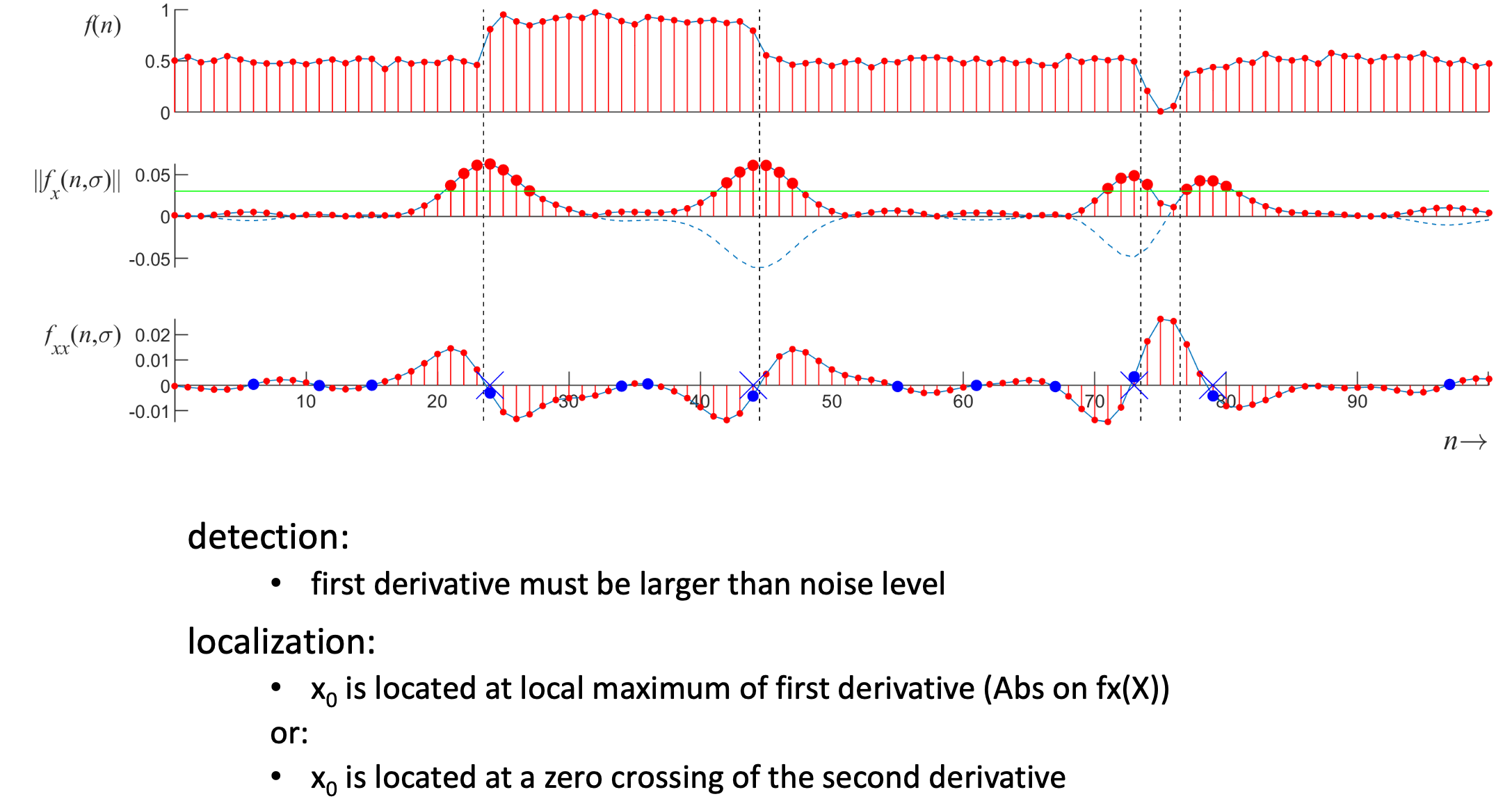
Finding Zero Crossings

• Slope of zero-crossing of $L(x,y)$ which is the result of $LoG$ convolution.
  • $slope=\sqrt{(\frac{dL}{dx}{)}^2+(\frac{dL}{dy}{)}^2}$
• To mark an edge
  • compute slope of zero-crossing
  • Apply a threshold to slope

Canny Edge Detector

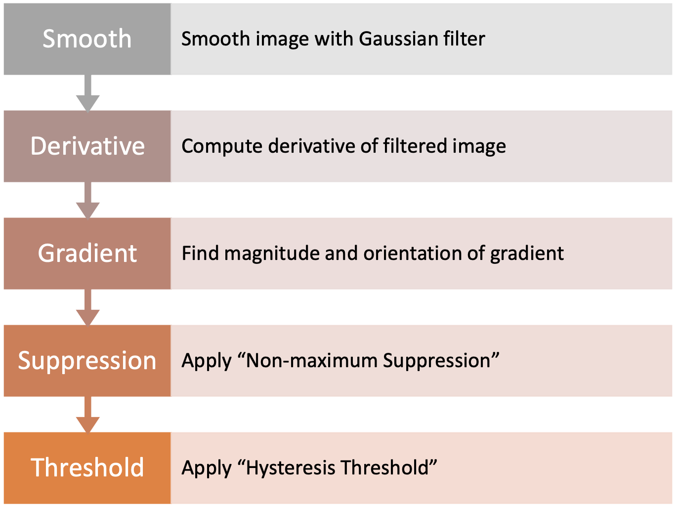
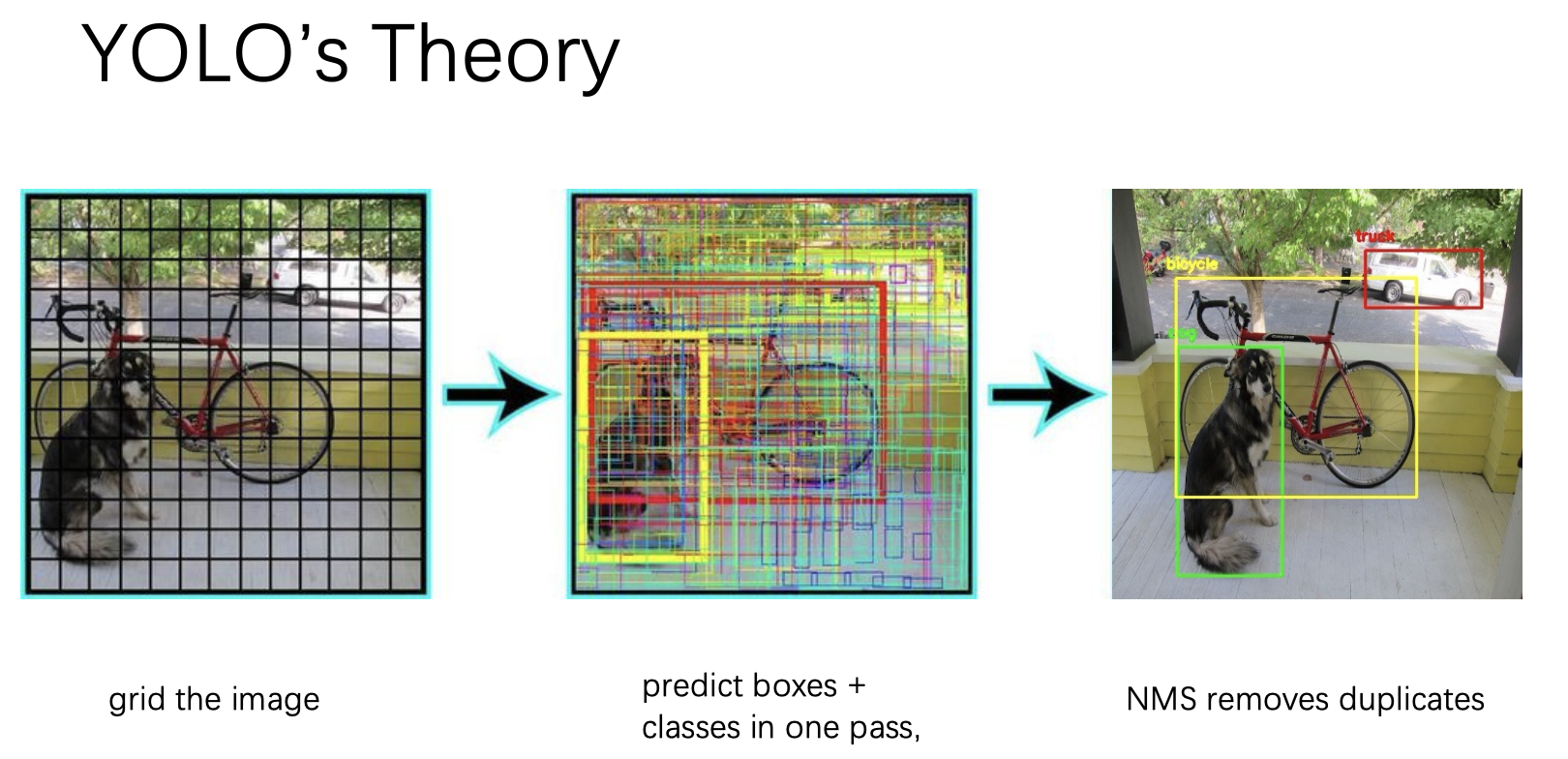
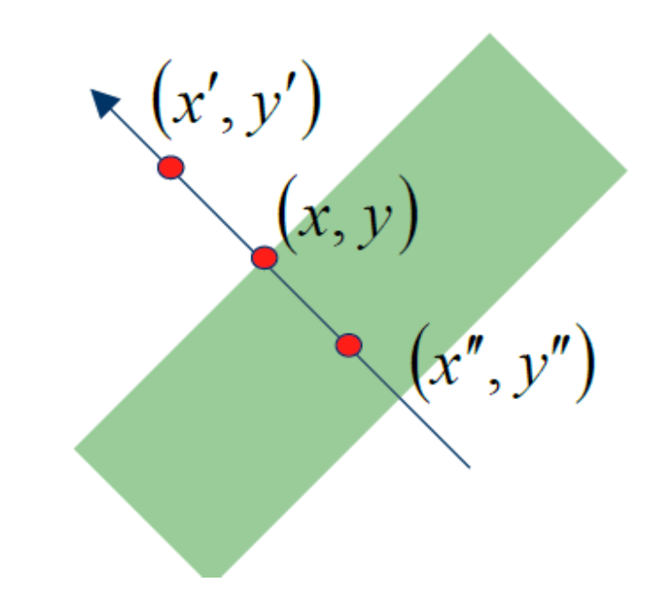
Non-Maximum Suppresion (NMS)

NMS

• We wish to mark points along the curve where the magnitude is largest. We can do this by looking for a maximum along a slice normal to the curve (non-maximum suppression)
• These points should form a curve. There are then two algorithmic issues: at which point is the maximum, and where is the next one?

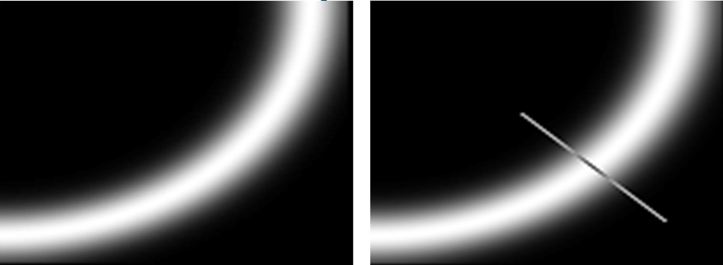
• Suppress the pixels in $|\nabla S|$ which are not local maximum.
• $x’$ and $x’’$ are the neighbors of $x$ along normal direction to an edge.

$$M(x,y)=\{\begin{array}{ll}|\nabla S|(x,y)& \text{if }|\nabla S|(x,y)>|\nabla S|(x^{\prime },y^{\prime })\\ & \text{and }|\nabla S|(x,y)>|\nabla S|(x^{\prime \prime },y^{\prime \prime })\\ 0& \text{otherwise}\end{array}$$

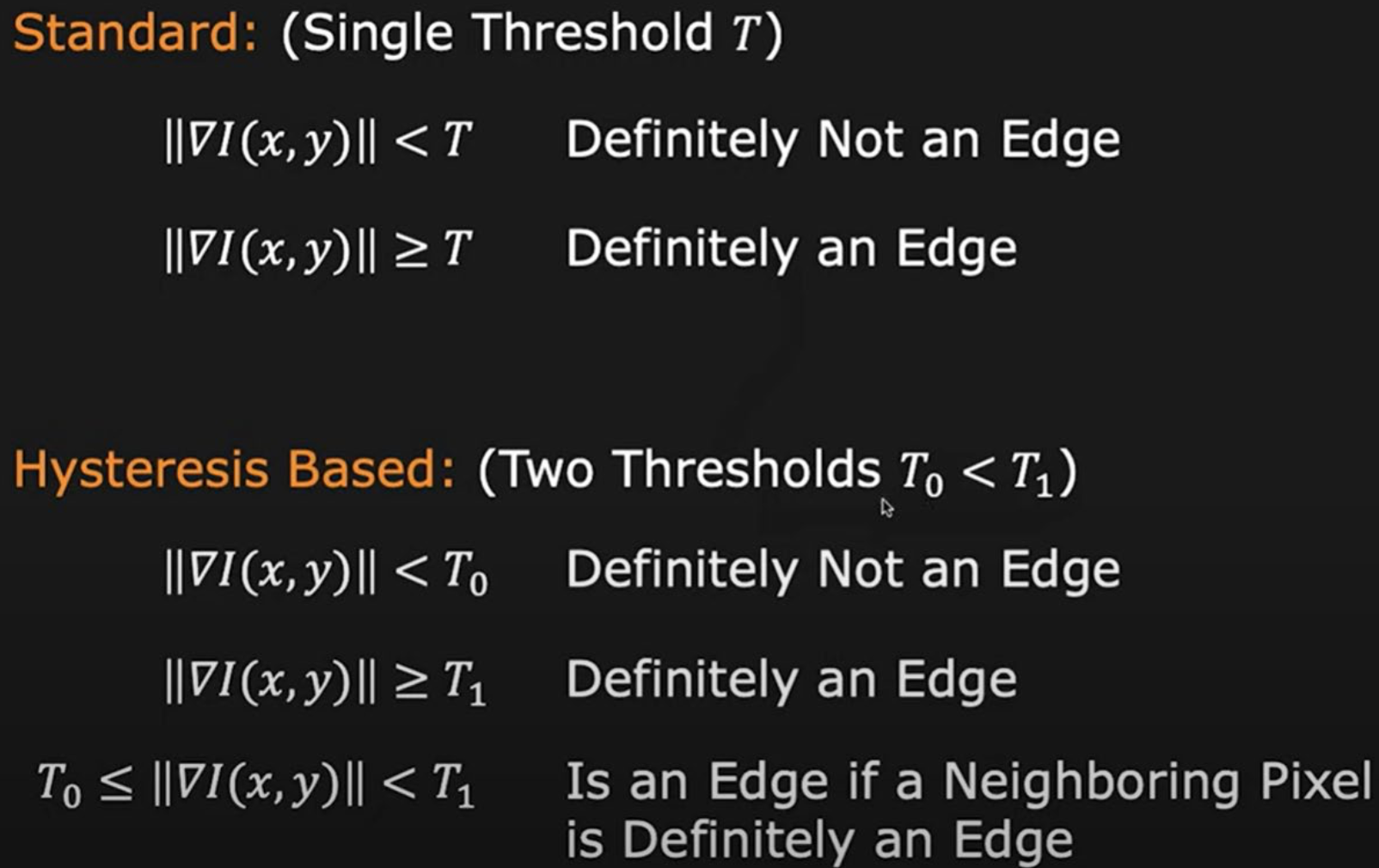
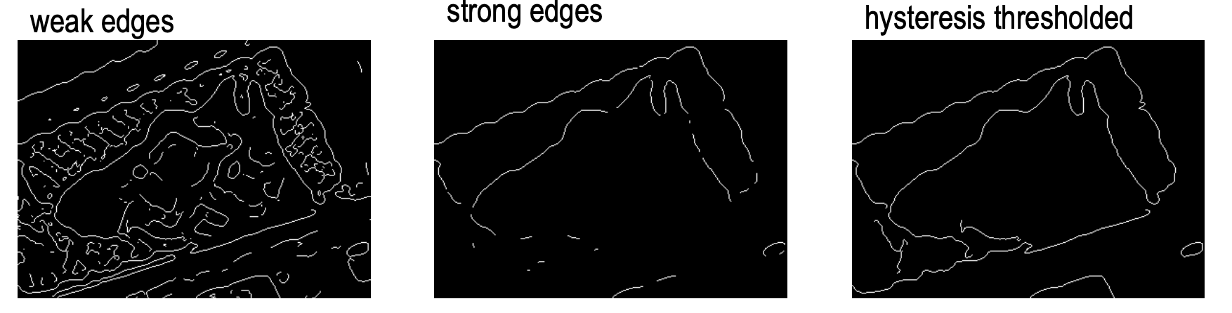
Hysteresis Thresholding

Summary

• Use two different thresholds to define strong edges and weak edges.
• Weak edges are accepted only if they are connected to at least one strong edge element.

Lecture 6: Geometric Transformations

Linear Transformations

• Scaling, rotation and reflection can be combined as a 2D linear transformation
• Preserve shapes

Linear transformations are combinations of

• Scale,
• Rotation,
• Shear,
• Mirror

Properties of Linear Transformations

• Origin maps to origin (not in translation)
• Straight lines map to straight lines
• Parallel lines remain parallel
• Ratios are preserved

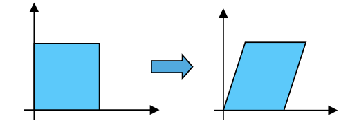
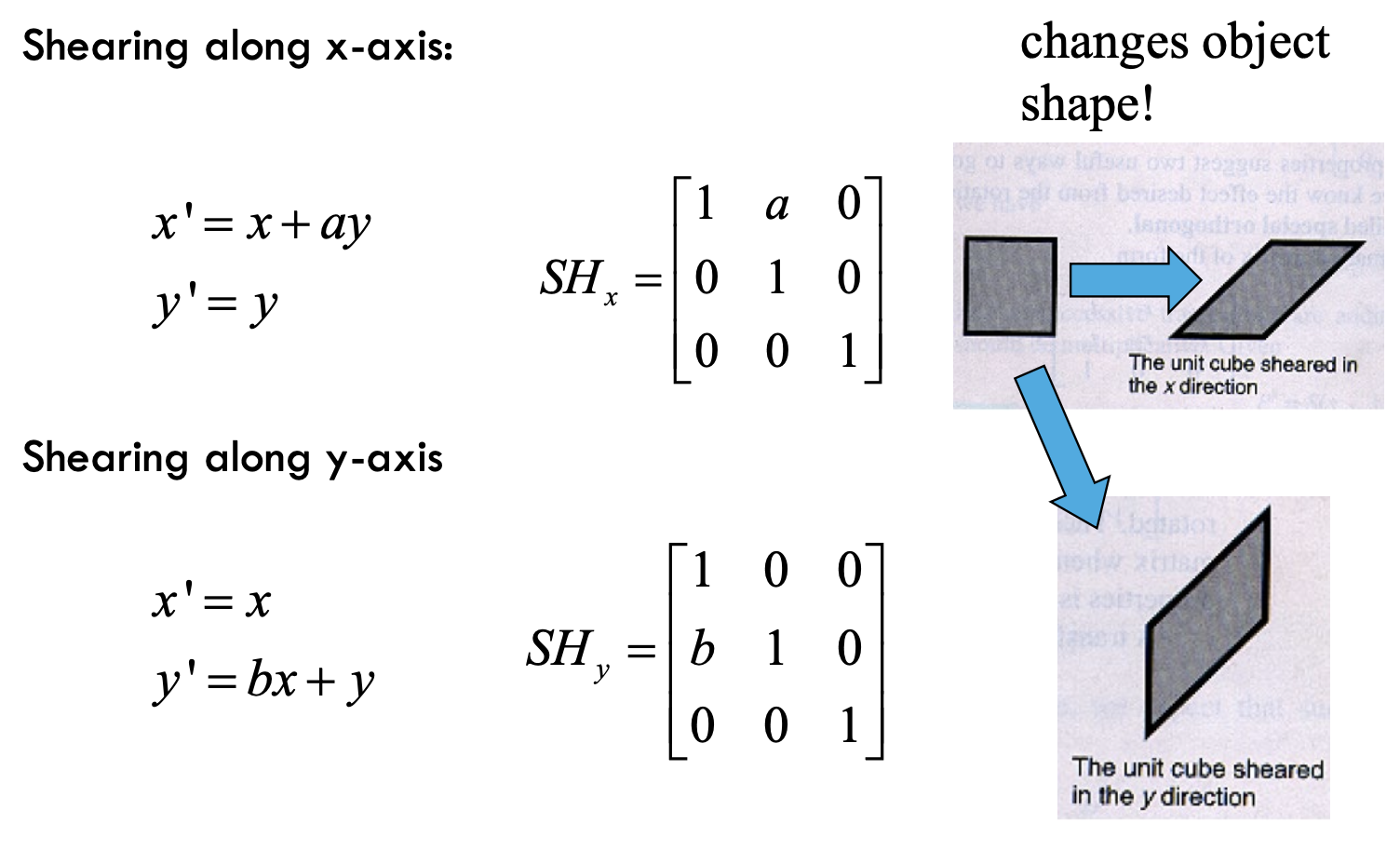
Shearing

• changes object shape

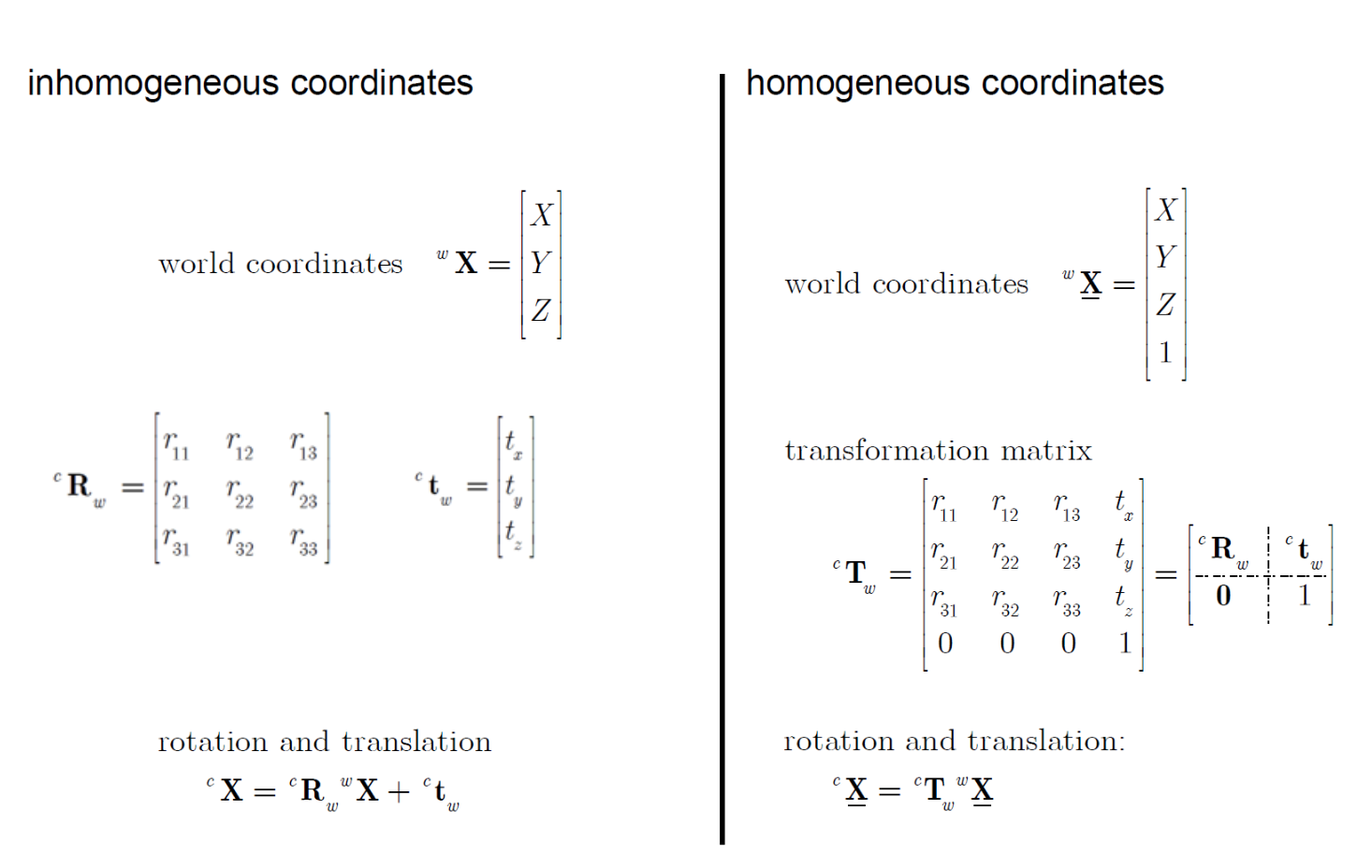
Homogenous Coordinates

Homogenous Coordinates

• Add an extra dimension to coordinates: $(x,y)\Rightarrow \left[\begin{array}{c}x\\ y\\ 1\end{array}\right]$ which allows for perspective projections and other projective transformations to be treated as linear transformations that can be represented by matrice.
• Used to simplify and combine transformations like translation, rotation, and scaling into single matrix multiplications

Affine Transformations

• any transformation with last row $[0,0,1]$ we call an affine transformation

• Affine transformations are combinations of
  • Linear Transformations
  • Translations

Properties of affine transformations

• Origin does not necessarily map to origin
• Lines map to lines
• Parallel lines remain parallel
•  Ratios are preserved

Projective Transformations (Warping)

Properties of projective transformations

• Origin does not necessarily map to origin
• Lines map to lines
• Parallel lines do not necessarily remain parallel
• Ratios are not preserved

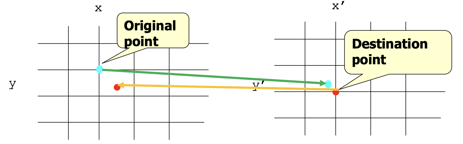
Mapping

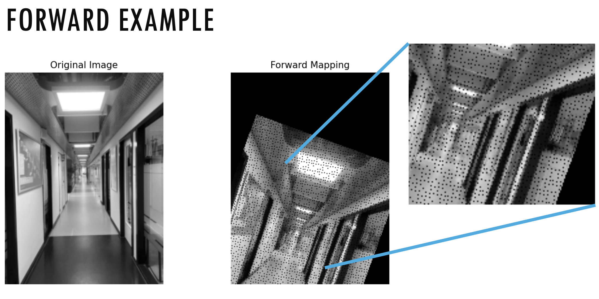
Forward Mapping

• From source image $\to$ destination image
• Not every destination pixel is guaranteed to be hit by some source pixel. As a result, some pixels in the destination image remain empty, creating gaps or holes.
• Source and destination images may not be the same size
• Output locations may not be integer values

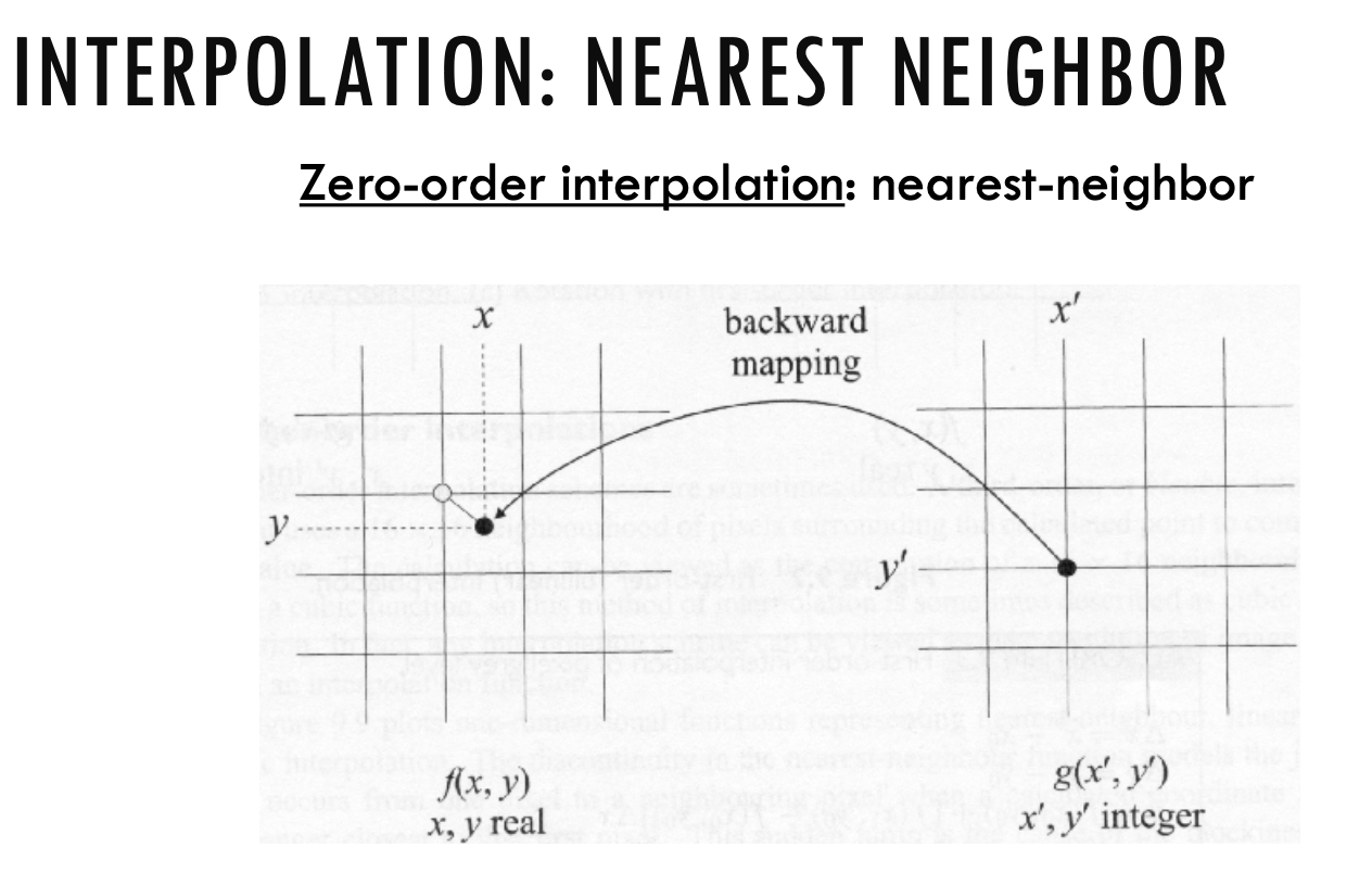
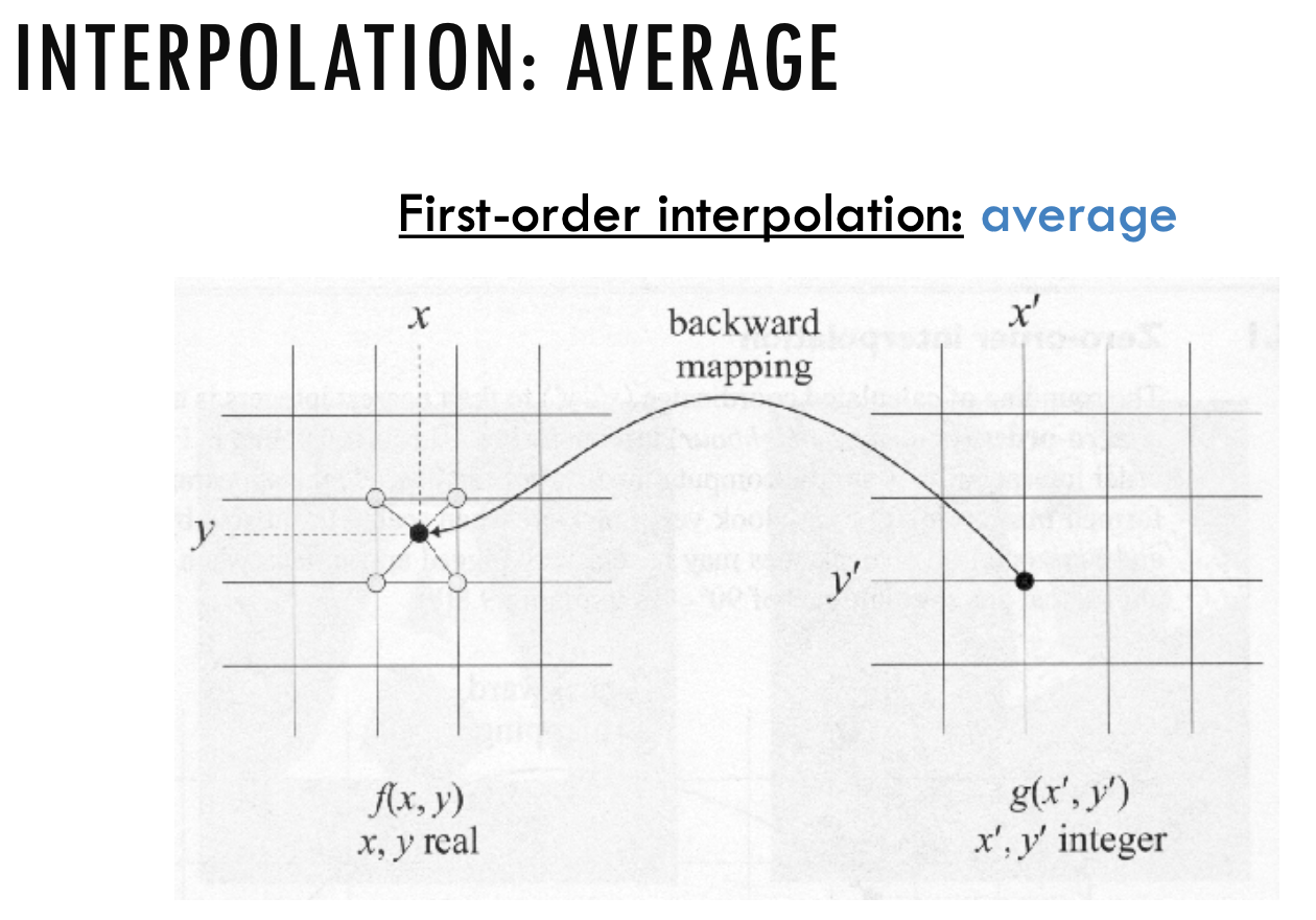
Backward Mapping

• From destination image $\to$ source image
• No gaps (through inverse mapping). To assign intensity values to these locations, we need to use some form of intensity interpolation

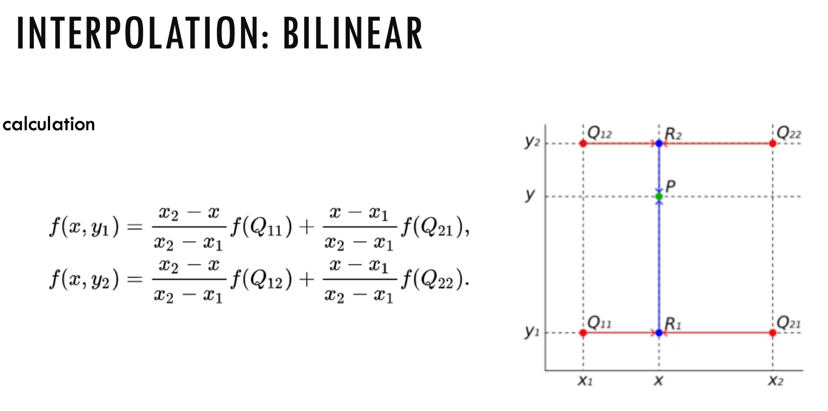
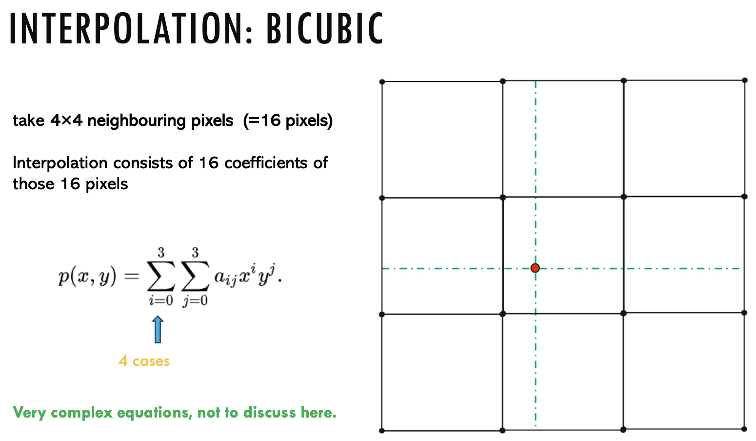
Interpolation Methods

Lecture 7: Camera Model and Calibration

Homogenous Coordinates in 2D

• Homography: a projective transformation
• Undoing a perspective distortion in an image
• transformed lines are still lines
• lines that share a common vanishing point keep on sharing a vanishing point
• distances are not preserved
• angles are not preserved

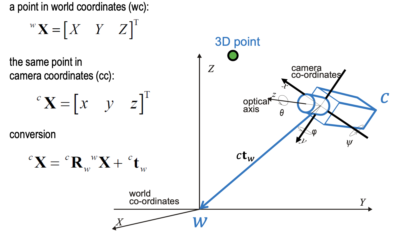
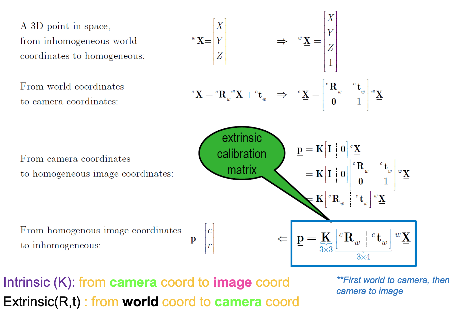
World to Camera coordinates

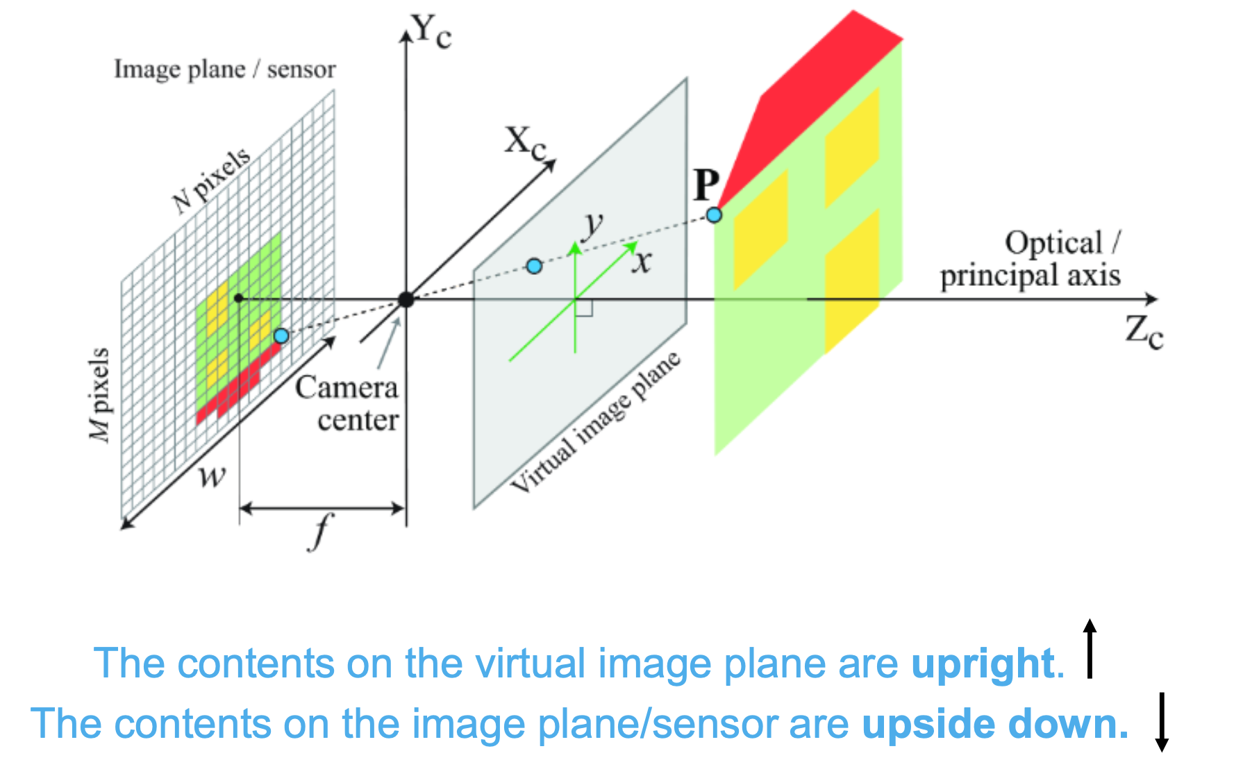
Perspective Projection of a camera

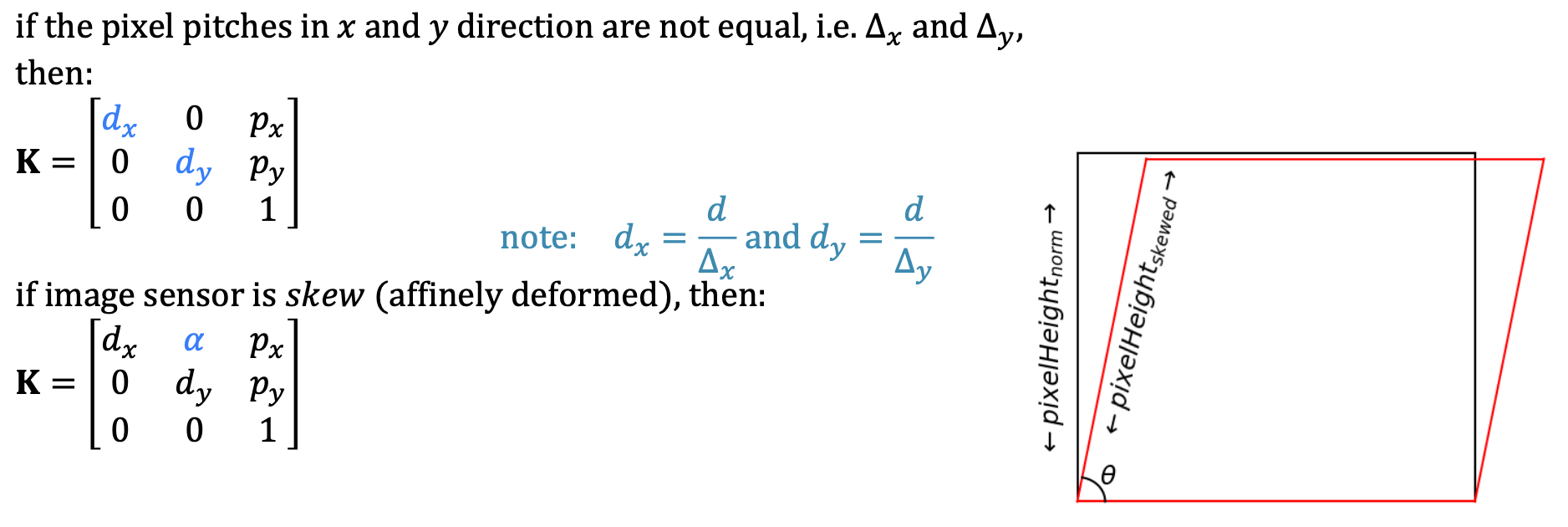
Intrinsic Camera Model

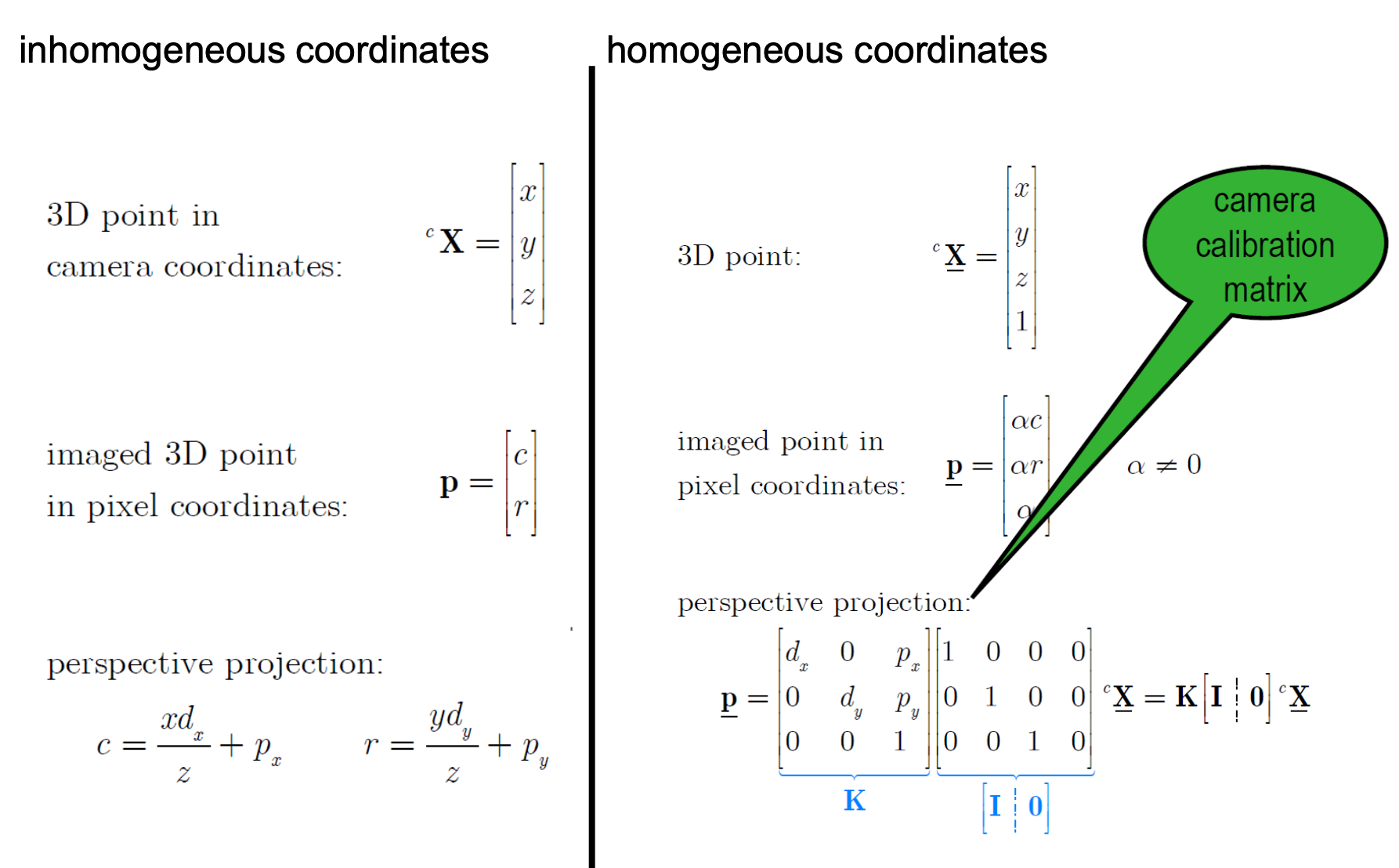
• $r,c$ are pixel coordinates, we want to calculate them
• $p_x$, $p_y$ are principal point = image center
• $d_x,d_y$ are distances between pixels (focal distance)

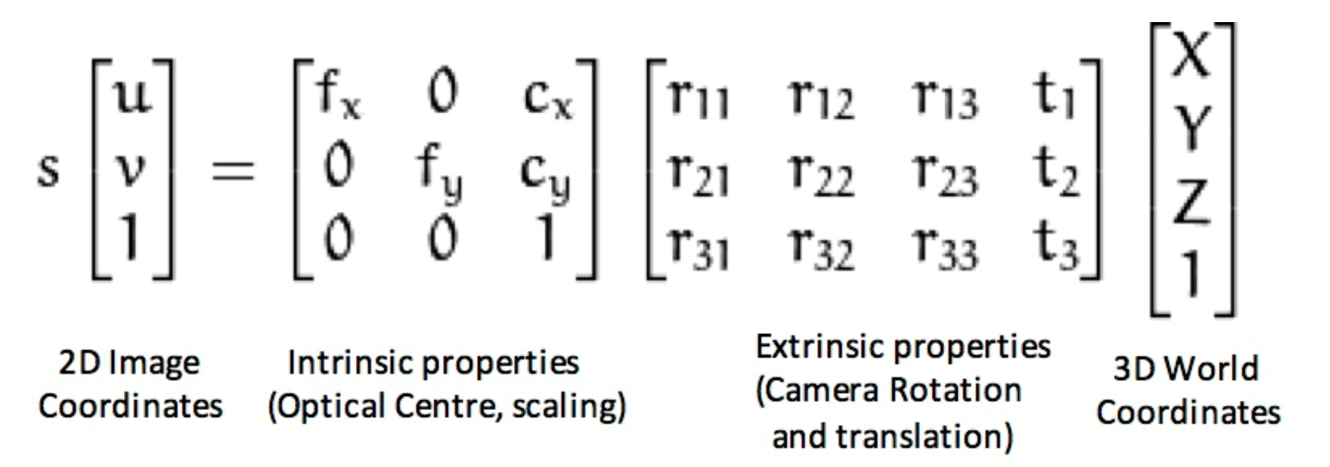
• $f_x,f_y$ are the focal length
• $c_x,c_y$ are the principal point
• $s$ is the skew efficient
• These parameters map 3D camera coordinates to 2D image coordinates.

As a summary

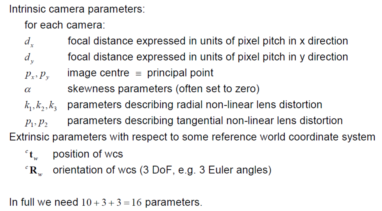
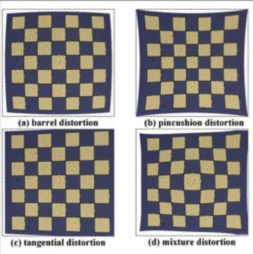
Distortion

Radial Distortion

• parameters $k_1,k_2,k_3$
• This type of distortion usually occur due unequal bending of light. The light ray gets displaced radially inward or outward from its ideal location before hitting the image sensor.
• The rays bend more near the edges of the lens than the rays near the centre of the lens.
• Due to radial distortion straight lines in real world appear to be curved in the image.
• Barrel distortion(negative radial displacement), Pincushion distortion(positive radial displacement)

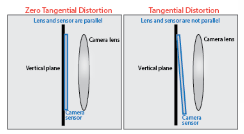
Tangential Distortion

• parameters $p_1,p_2$
• This usually occurs when image screen or sensor is at an angle w.r.t the lens. Thus the image seem to be tilted and stretched.

Type of distortions

Lecture 8: Template matching & line detection

Mind these

• position
• size
• orientation
• background
• contrast

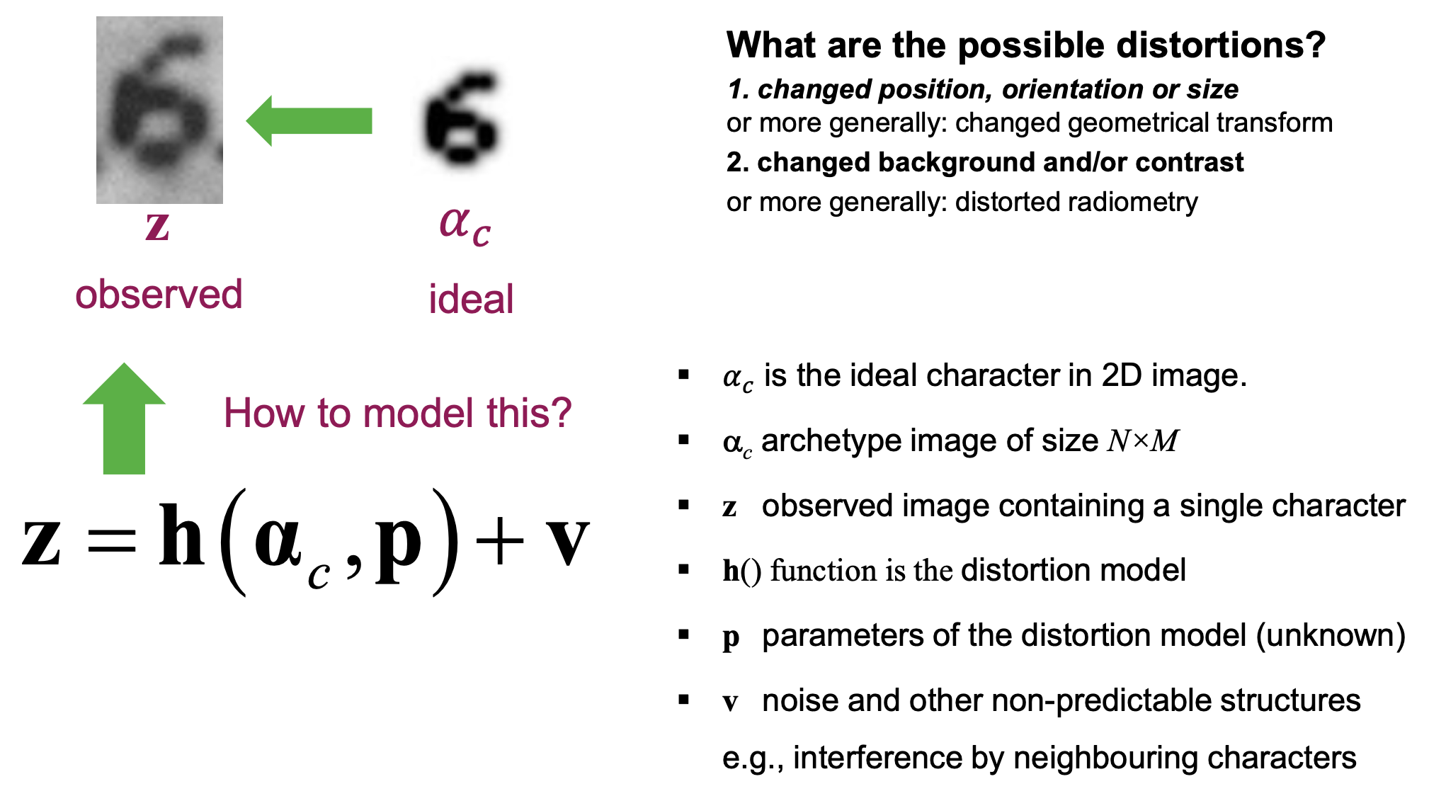
The template is an iconic archetype of the object that we are looking for.

Template Matching

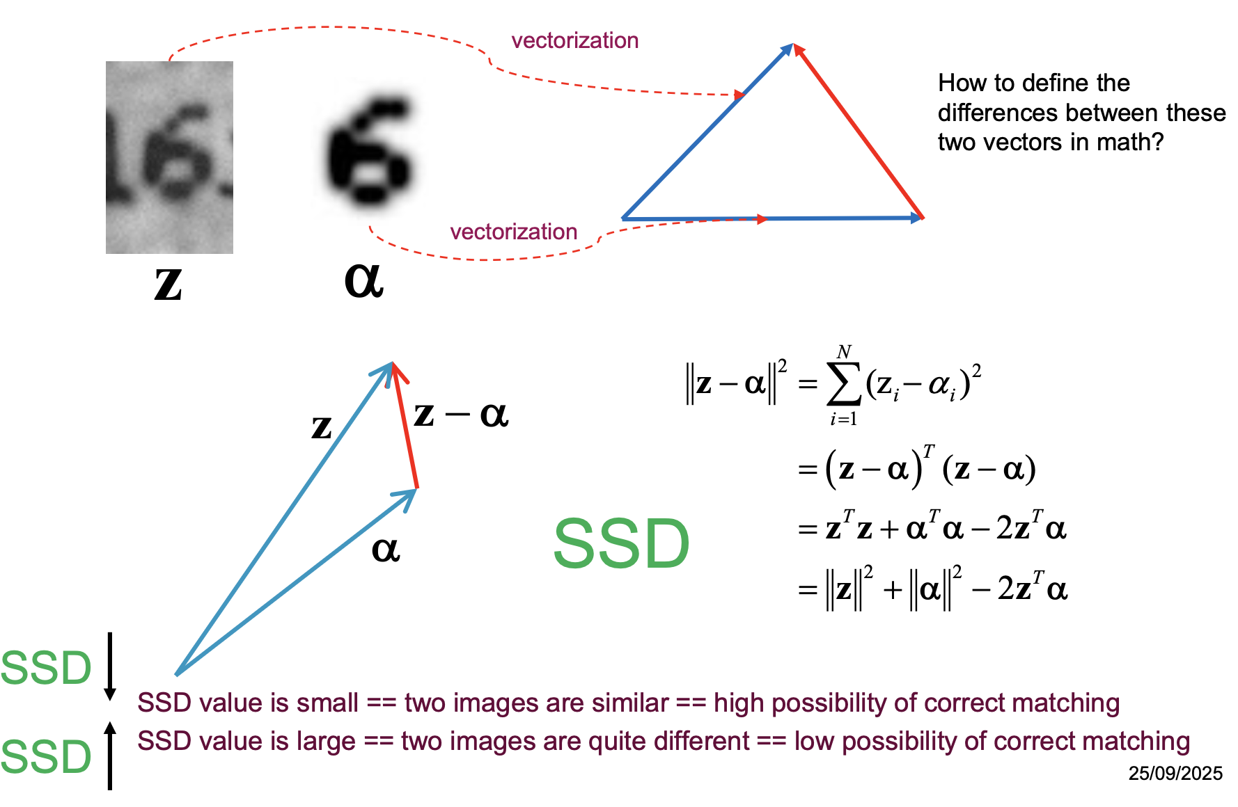
Can we find locations in the image where locally the image “looks like” the archetype? — We need to define what “looks like” is.

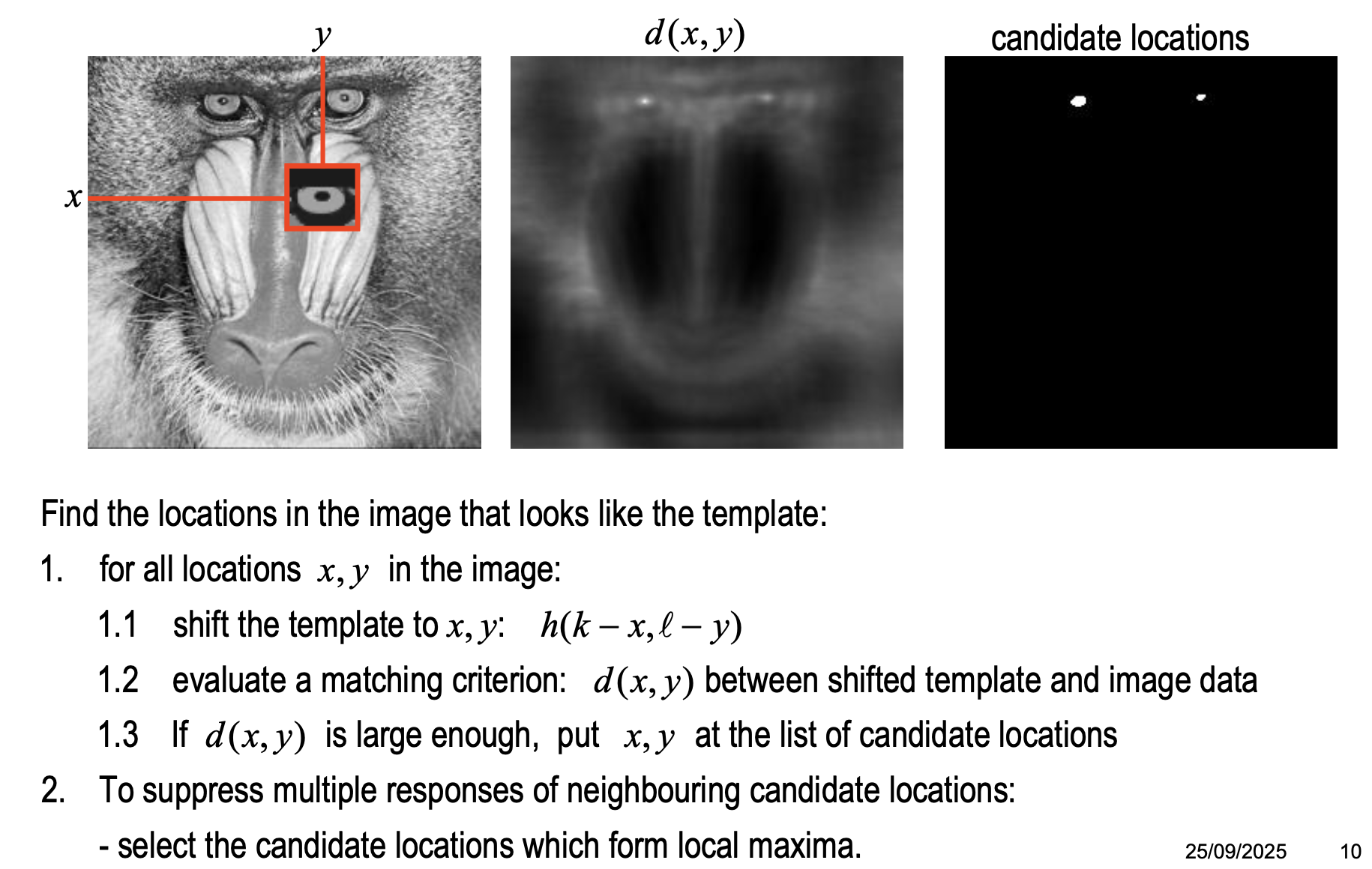
Matching Criterion: SSD (Sum of squared differences)

• type of distortion: unknown shifted position (𝑝, 𝑞)

NCC (Normalized Cross Correlation)

• type of distortion: unknown amplitude: 𝐴

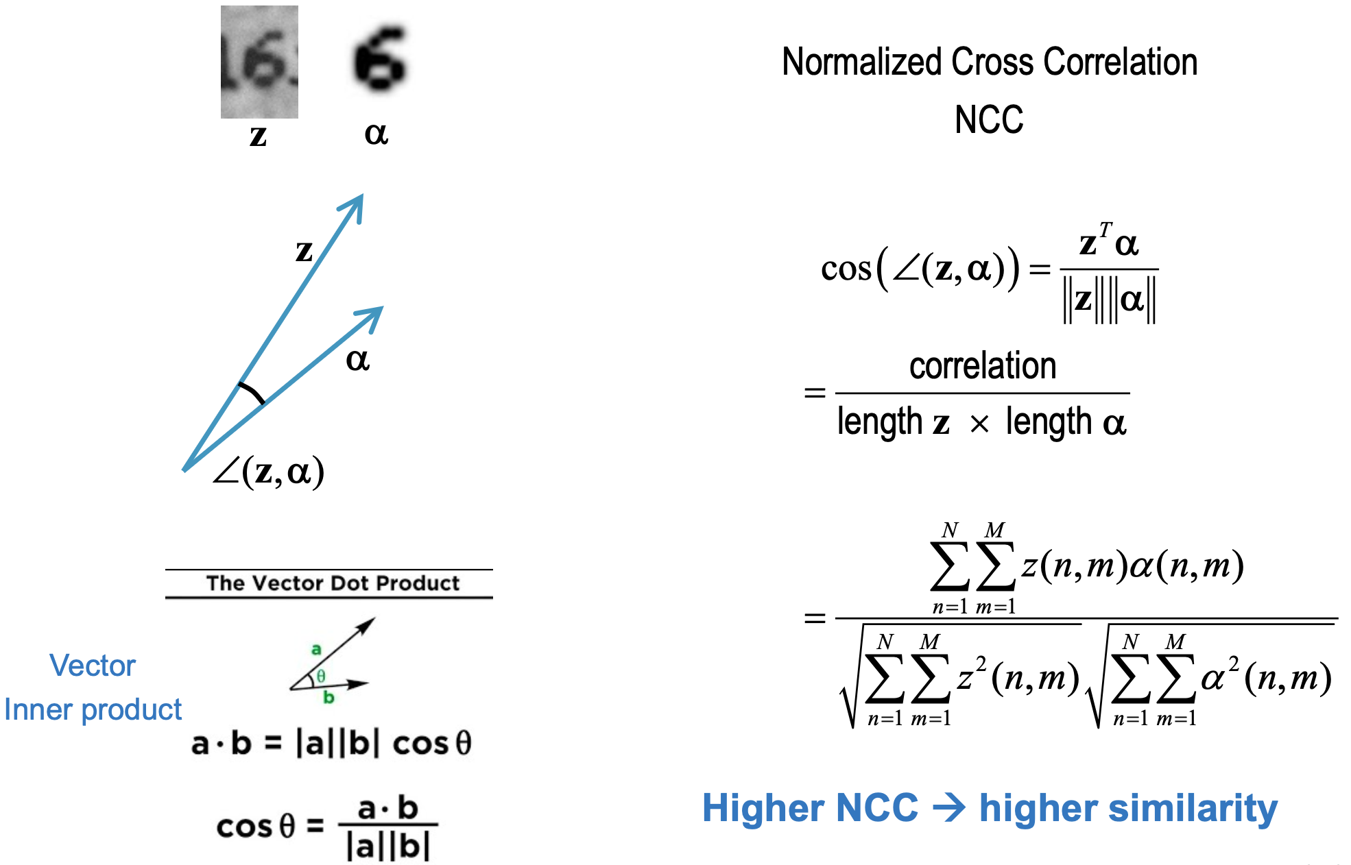
• Normalization solution:
  • estimate from bg
  • neutralize bg by subtraction (Normalize background in observe image and background in template image)

Line Detection

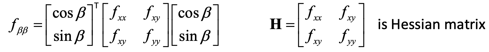
β = direction across line element

• Idea: try normalization wrt orientation — this will be very computationally expensive (correlation with line templates)

  • estimate locally the orientation of the line: β
  • rotate the template over an angle of –β
  • apply locally template matching

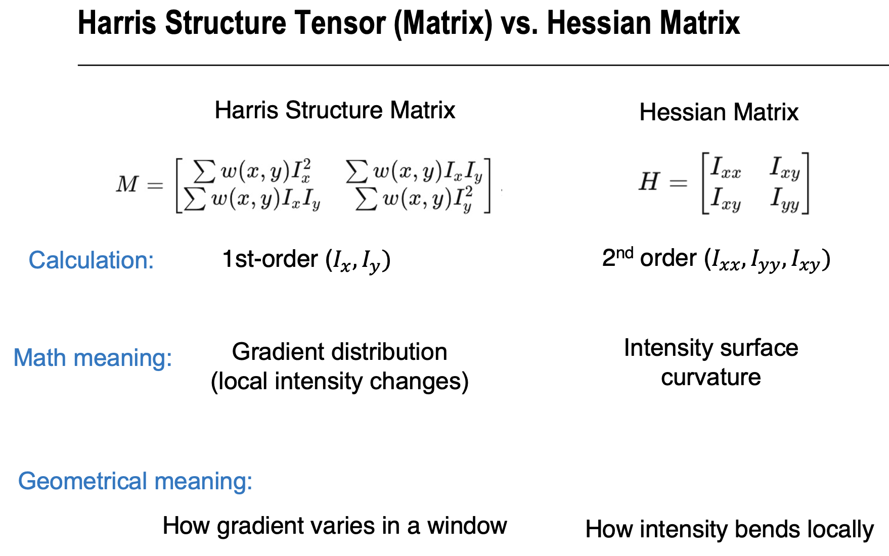
• Solution: 2nd directional derivative in direction β (eigenvalues of Hessian matrix)

  • β corresponds to the dominant eigenvector 𝐯 of the Hessian matrix
  • The maximized $f_{\beta \beta }(x,y)$ equals the eigenvalue of the Hessian matrix

Lecture 9: Detection and tracking of interest points

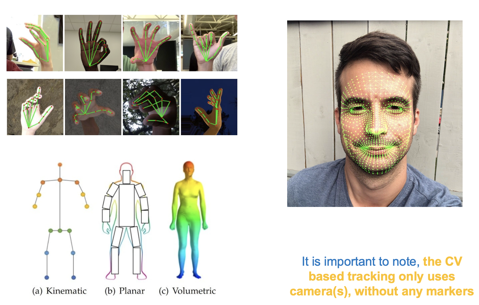
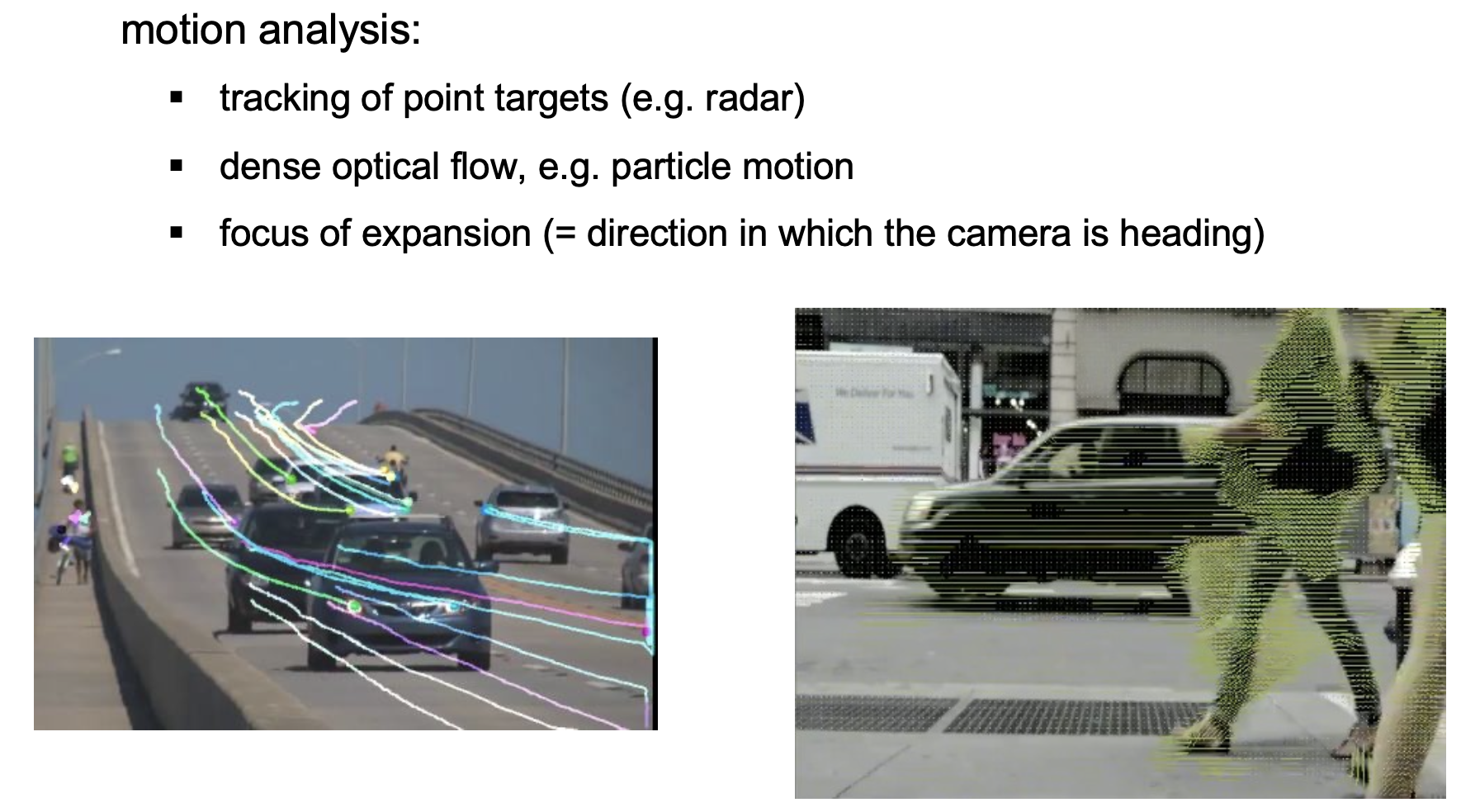
Applications

• motion analysis
• range imaging
• object detection and parameter estimation
• point cloud

Harris Corner Detection

Harris’ first improvement

• Make the function less noise−sensitive by averaging over a neighborhood
• New term with average window
• $E(p,q)$ defines and ellipsoid. Its contour lines are ellipses in the $(p,q)$ plane
• The shape of the ellipsoid is determined by ${\lambda }_1$ and ${\lambda }_2$

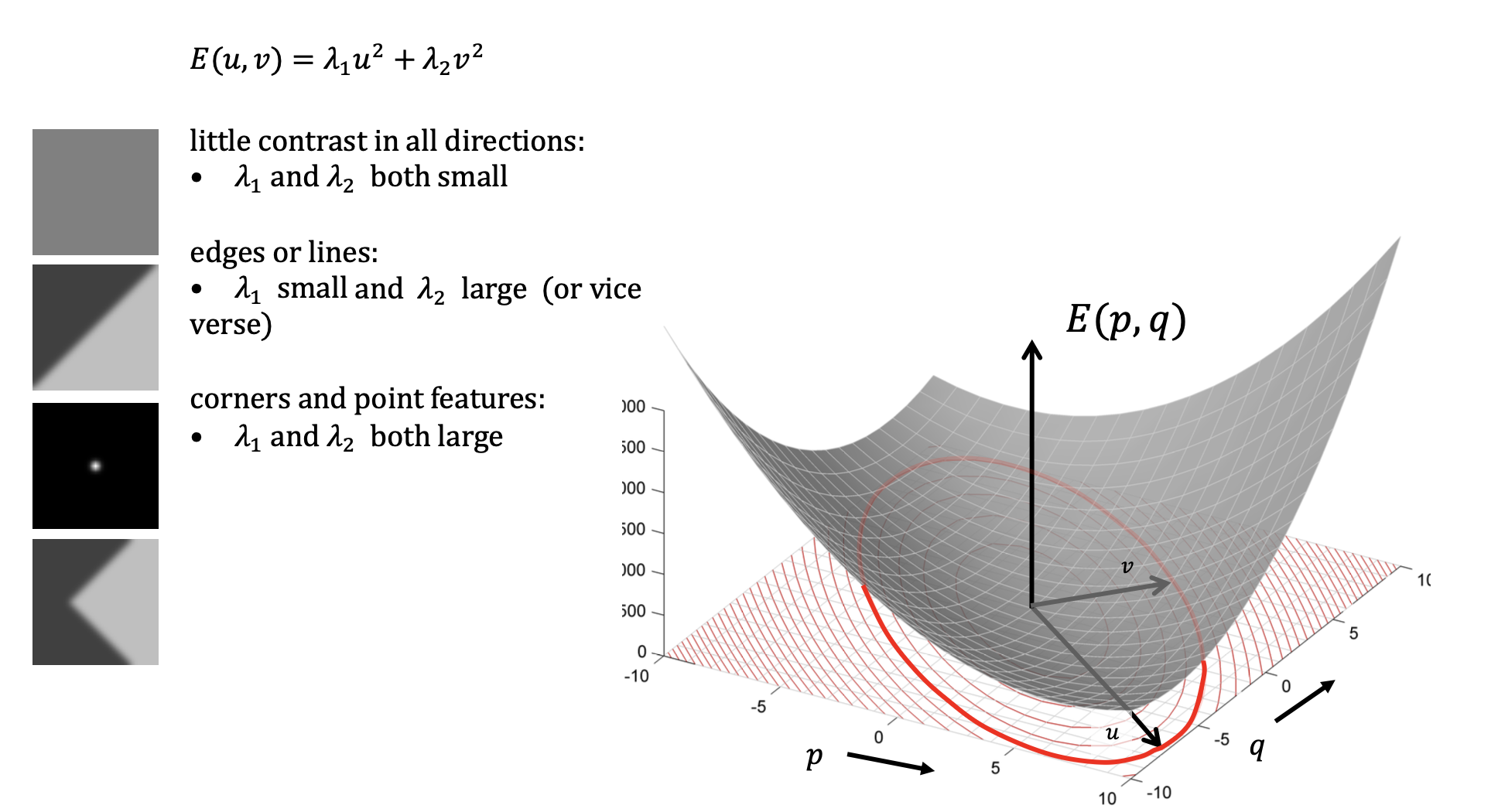
Harris’ second improvement

• A point is an interest point iff $E(p,q)$ is fast increasing for any combination of $p,q$. That is, the ellipsoid must be peaked.
• Therefore, both ${\lambda }_1$ and ${\lambda }_2$ must be large.

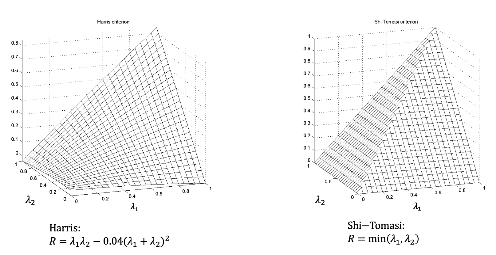
Harris criterion for an interest point

${\lambda }_1{\lambda }_2-0.04({\lambda }_1+{\lambda }_2{)}^2>threshold$

Shi−Tomasi ciriterion for an interest point (1994)

$min({\lambda }_1,{\lambda }_2)>threshold$

Harris’ third improvement

• Use a Gaussian weight function (less noise-sensitive): $w(n,m)=\exp (-\frac{n^2+m^2}{2{\sigma }^2})$

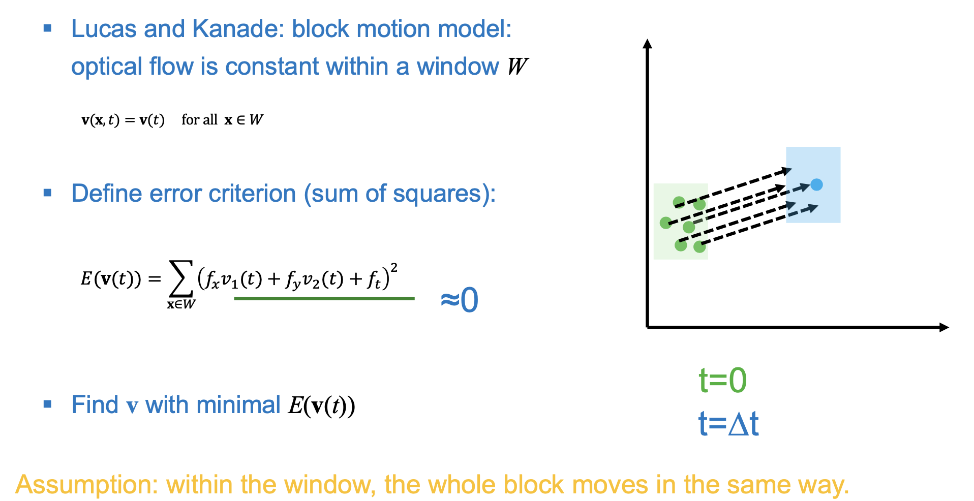
Lucas-Kanade: Point Tracking

Tracking

• Given two or more images of a scene, find the points in the second and next images that corresponds to the set of interest points in the first image

Optical Flow $\ne$ Motion Field

• Optical flow = appearance model
• Motion field = physical world

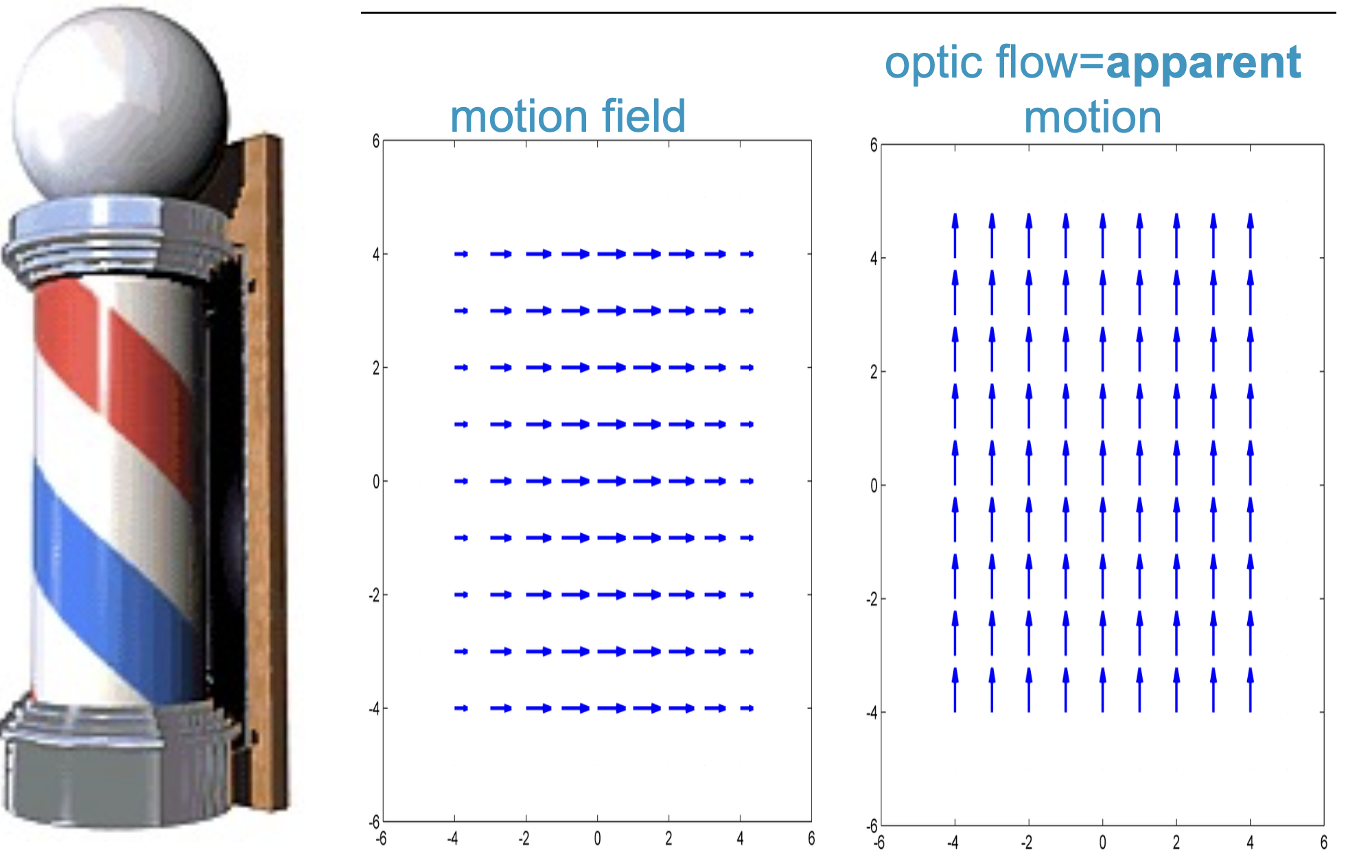
For the example above, think about how the lines go up as the result of the rotating pole inside.

Optical Flow

• Constant brightness assumption: if the intensity of a pixel stays the same over a duration $t$, then it’s derivative is 0 and thus stationary (?)
• $v(\mathbf{x},t)$ is the apparent 2D motion (= optical flow) of the image at position $\mathbf{x}$ and time $t$.
• $\mathbf{x}=(x,y)$

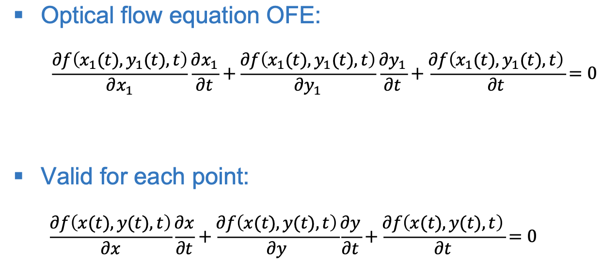
• Minimization of $E(v,t)$:
  • equating partial derivatives to zero
  • solving for $v(t)$
  • The two eigenvalues of M must be large

Discrete time

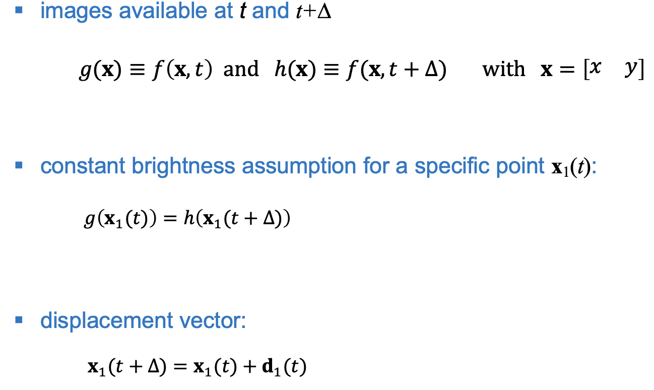
• We minimize SSD with respect to d: $\frac{dSSD(d)}{dd}=0$

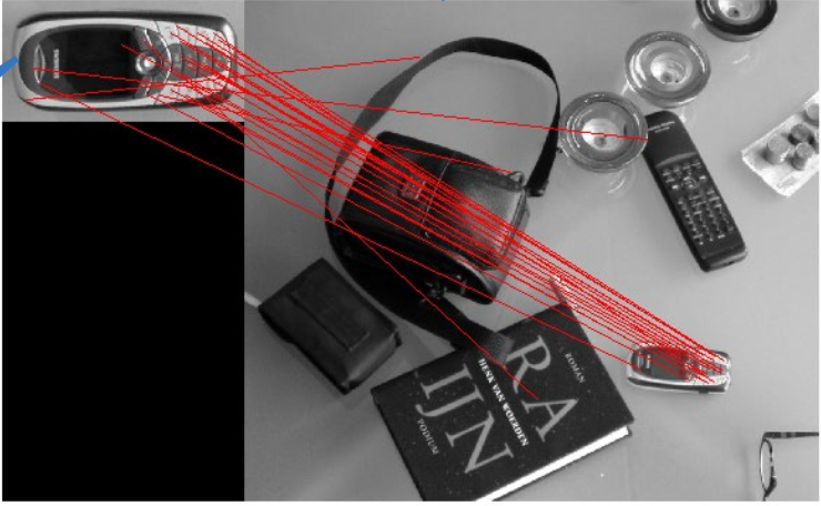
Lecture 10: Key point detection and matching

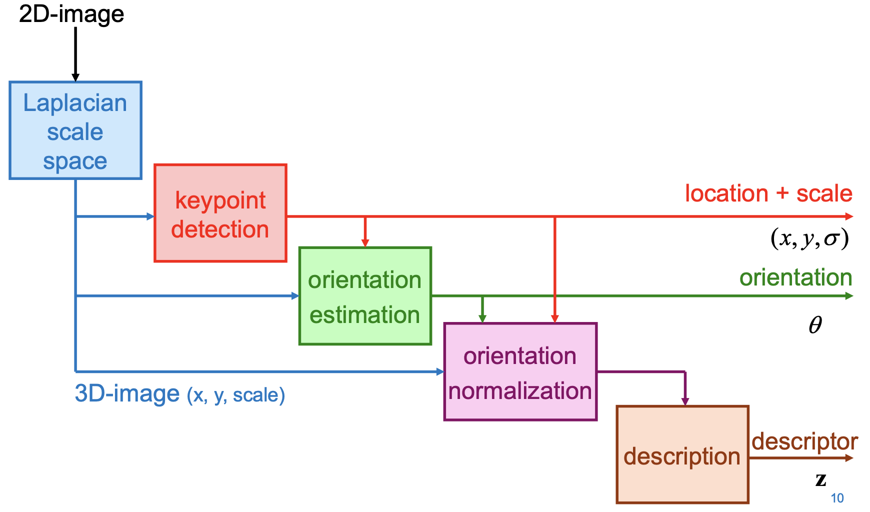
SIFT (Scale Invariant Feature Transform)

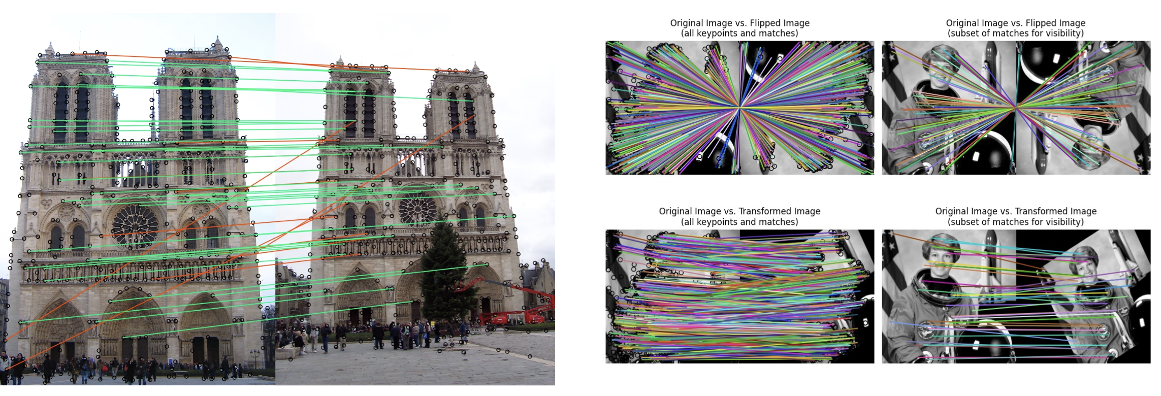
Keypoints in SIFT

• set of point features defined in an image
• each key point is attributed with:
  • the local orientation
  • the scale
  • a descriptor (used to identify the local neighbourhood)
• useful properties:
  • invariant to image translation, rotation and scaling
  • invariant to contrast and brightness
  • partially invariant to the 3D camera viewpoint
  • distinctive
  • stable
  • noise insensitive

• zooming the image by a factor $a$:
  • does not change the location of a keypoint
  • changes the scale of a keypoint by a factor $1/a$

Laplacian of a Guassian (Inverted Sombrero)

$LoG(x,y,\sigma )=\Delta gauss(x,y,\sigma )=\frac{x^2+y^2-2{\sigma }^2}{2\pi {\sigma }^6}\exp \left(-\frac{x^2+y^2}{2{\sigma }^2}\right)$

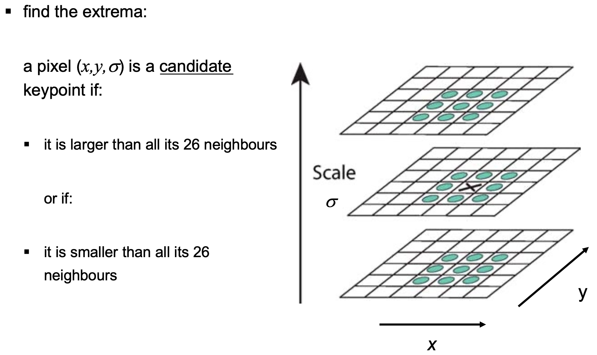
Detection of candidate keypoints

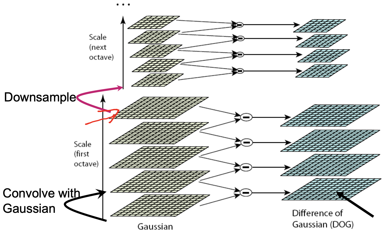
Efficient implementation of the LoG

• approximation of LoG by differences of Gauss (DoG): $LoG(x,y,\sigma )=△gauss(x,y,\sigma )$
• cascade of Gaussians

• Representations for matched keypoints are done through:
  • adjacency matrix
  • bipartite graphs
  • table of edges
  • table of pointers
  • distance table

Applications

• image stitching
• stereo rectification
• landmark detection and matching for visual SLAM
• object recognition

Lecture 11: 3D Vision. Binocular Vision

• Dense stereo

  • reconstruction of 3D surface models of objects

• Sparse stereo

  • 3D information on a small number of points:
    • finding the 3D positions of the points from multiple images
    • finding the 3D pose of a camera relative to the points
    • finding the pose of the camera relative to another camera
    • visual SLAM: finding both the poses of cameras and the 3D positions of points

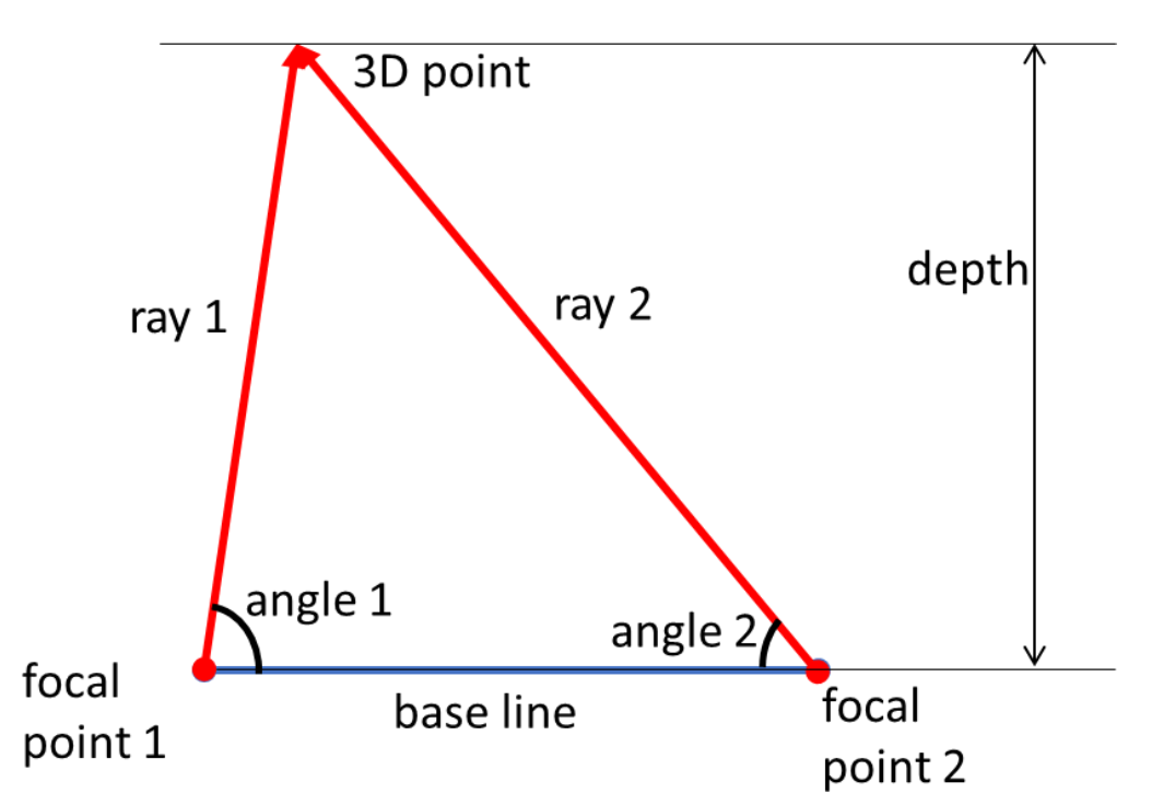
Triangulation

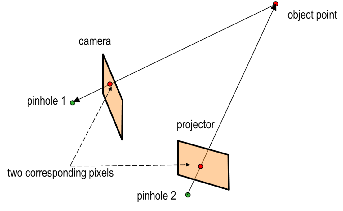
• Key relations:
  • Triangulation (base line, two rays)
  • Correspondence: representation of 3D point: $X^1=R_2^1{X}^2+t_2^1$

Epipolar Geometry

• How to find corresponding pixels?
• How to reconstruct the 3D position of object?

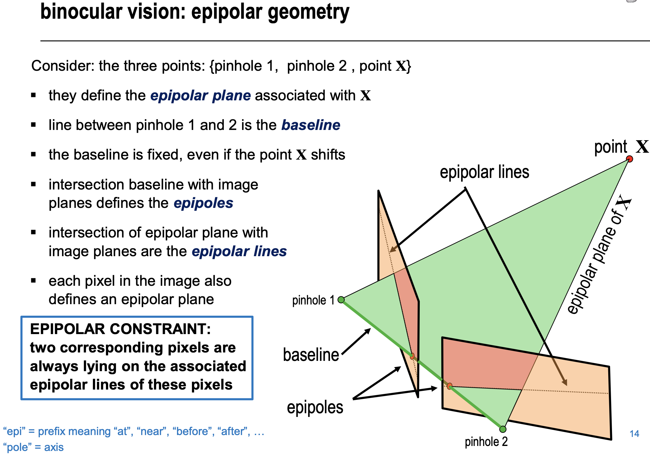
• Epipolar constraint expressed with Essential Matrix: $X_2^{T}E{X}_1=0$

• E is the Essential Matrix: $E=R_1^2[t_2^1{]}_x$

• Epipolar constraint in pixel coordinates: fundamental matrix

  • ${}^1\underline{\mathbf{p}}=K_1{X}^1$
  • ${}^2\underline{\mathbf{p}}=K_2{X}^2$
    • Substitution in $X_2^{T}E{X}_1=0$ yields: ${}^2{\underline{\mathbf{p}}}^{\top }{\mathbf{K}}_2^{-\top }\mathbf{E}{\mathbf{K}}_1^{-1}{}^1\underline{\mathbf{p}}=0$
  • define $F={\mathbf{K}}_2^{-\top }\mathbf{E}{\mathbf{K}}_1^{-1}$ then:
    • Epipolar constraint in pixel coordinates:
      • ${}^2{\underline{\mathbf{p}}}^{\top }{F}^1\underline{\mathbf{p}}=0$
      • $F$ is the fundamental matrix

Rectification

• geometrical transformation of the images such that the epipoles are moved to infinity in the row-direction.
• simplifies the correspondence problem to a simple 1-D search along rows.
• needs calibration matrices K1 and K2, and fundamental matrix F

Rectification Steps

1. determine the rotation axis and rotation angle between camera 1 and camera 2
2. rotate camera 1 around this axis over half of the angle in counterclockwise direction
3. rotate camera 2 around this axis over half of the angle in the other direction
4. determine the direction between x-axis of the cameras with respect to the baseline vector
5. using this direction, rotate the cameras such that their x-axis are aligned with the baseline vector
6. Equalize the calibration matrices of both cameras $K1==K2$

Disparity: difference of the seen pixels in two images

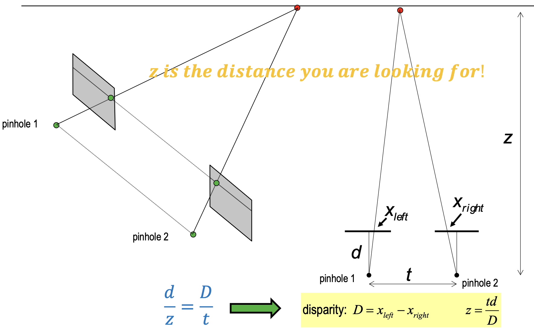
• Here we can see disparity and depth are inverse proportional
• Disparity is proportional to Baseline

Lecture 12: 1D signals and Depth Maps

1D Signals are very often seen in reality

• Earthquake
• Audio
• Temperature
• Bioelectrical Signal
• …

Monocular Depth Estimation

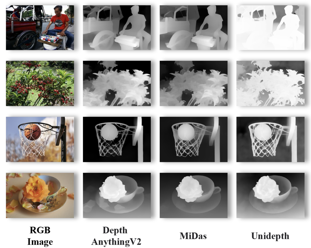
• Key Challenge: Scale Ambiguity
  • With only one image, absolute meters are unknown $\to$ models often predict relative depth that needs a later scale/shift alignment.

How does the human eye judge near vs. far?

• Occlusion: if one object blocks another, it’s closer.
• Relative / known size: the same object looks smaller when farther; familiar objects act as rulers.
• Linear perspective: parallel lines converge toward a vanishing point.
• Texture & contrast gradients: textures get denser and lower-contrast with distance (aerial haze).
• Lighting & shadows: shadow position/shape reveals spatial layout.
• Depth of field: in-focus plane is sharp; foreground/background blur more.
• Motion parallax: when you move, nearer objects shift faster across your view.